101
Honour Lectures /
Conférences honorifiques
Proceedings of the 18
th
International Conference on Soil Mechanics and Geotechnical Engineering, Paris 2013
where
y
is the minimum (yield) friction coefficient at very
slow shearing rates and
and
are the rate parameters; these
combine to give the rate-enhanced friction coefficient,
HB
.
Using the backbone consolidation curve shown in Figure 24
(Equation (40)) as the basis for pore pressure dissipation, the
excess pore pressure may be obtained by a convolution integral
of the form
'dt
e)'t(u q
D
)'t(v
*
u
t
0't
T/'TT2ln
m
50
(43)
where v and
u are both time varying functions and T' = c
v
t'/D
2
.
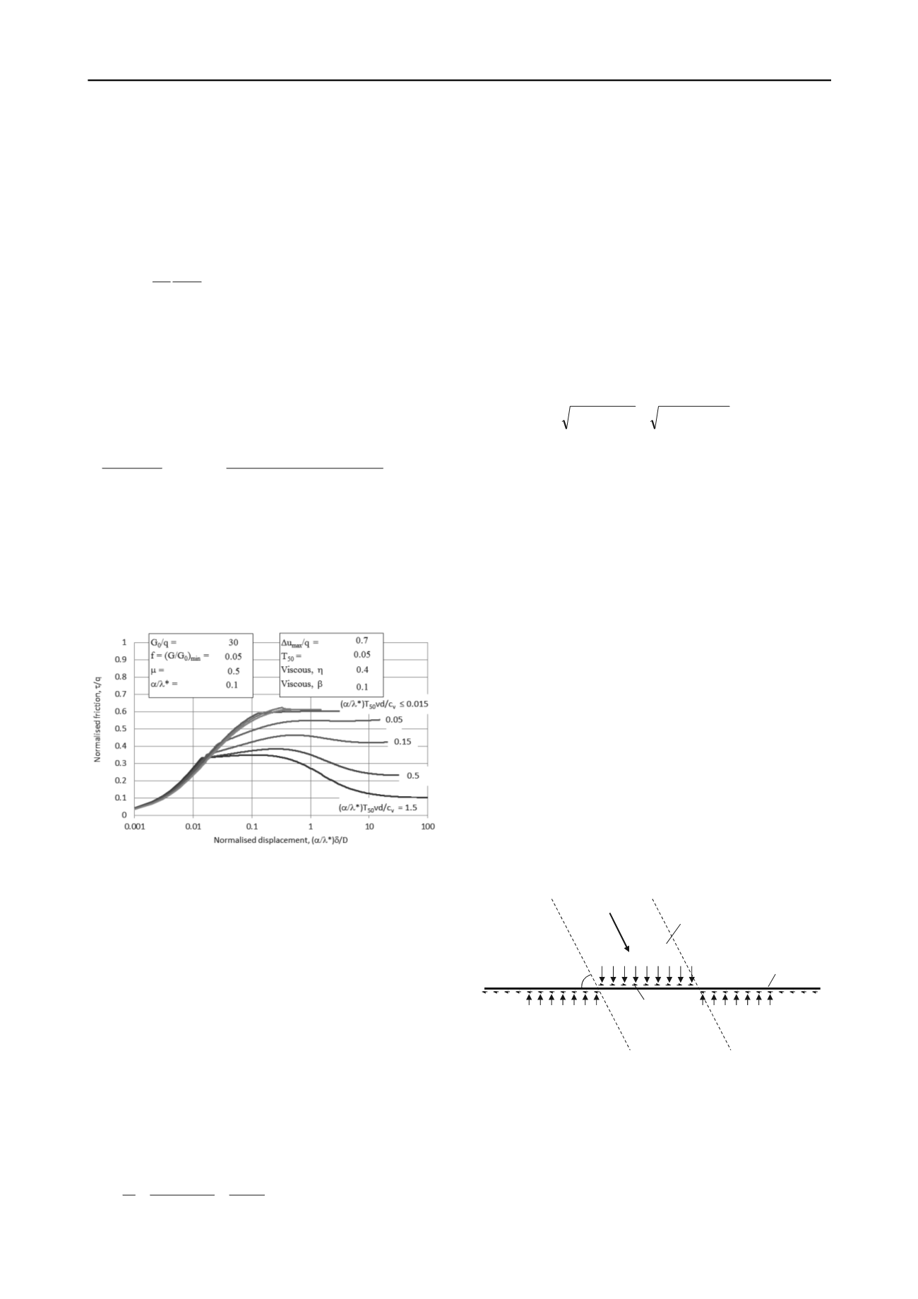
An example response is shown in Figure 25. Of particular
note is that after an initial transient stage, the normalised
friction,
/q, converges to a steady value that is a function of
velocity. At steady state, pore pressure generation due to
damage balances pore pressure dissipation due to consolidation.
The steady state friction was approximated as
v
50
HB
state
steady
c/ vDT* /
/24.01
1
1
q
(44)
Although this model of velocity and time-dependent axial
friction contains some speculative elements, such as the
proposed link between pore pressure generation and normalised
velocity, it provides a theoretical framework for design, and for
the planning of future model tests in the laboratory or field. It
also helps to resolve the apparent discrepancy between
conventional consolidation theory and experimental data.
Figure 25 Example axial response of pipeline incorporating damage
and strain rate (Randolph et al. 2012).
Axial stiffness
In addition to evaluating the limiting pipe-soil friction ratio, the
pre-failure axial stiffness of the pipeline is important as a
boundary condition for analysis of pipeline walking or the feed-
in to lateral buckles or debris flow impact. At an element level,
the axial stiffness (ratio of load transfer per unit length to axial
displacement) may be estimated by assuming a simple
distribution of shear stress around the perimeter of the pile,
similar to that for normal effective stress (Figure 22).
Consider a pipeline that is embedded to w/D = 0.5, and
where the shear stress resisting axial movement varies as cos
around the embedded section of the pipe. The shear stress will
also decrease inversely with radius from the pipe axis, in order
to satisfy equilibrium. Now assume a shear modulus for the soil
that varies proportionally with depth, z, according to G = mz. At
any radial position, the shear strain will therefore be
mr2
D
cosmr2
cosD
G
2
inv
2
inv
(45)
where
inv
is the shear stress at the pipe invert. Integrating this
with respect to r leads to the displacement at the pipe. The
resulting axial load transfer stiffness is then given by
mD k
a
(46)
For a partially embedded pipeline, this may be reduced by a
factor sin
m
, where
m
is defined in Figure 22. By comparison,
the vertical stiffness for a (surface) foundation of width Dsin
m
on similar soil would be given by k
v
= 2mDsin
m
(Gibson
1974). Hence the axial stiffness is about half the vertical
stiffness (a little lower, allowing for the embedded nature of the
pipeline, Guha 2013).
The axial load transfer stiffness may be combined with the
expression for the stiffness of a long pile (Equation (8)) in
order to yield the overall pipeline stiffness for axial motion:
mD EA k EA
K
pipe
a pipe
axial
, pipe
(47)
6.4
Impact forces from debris flows
Geohazard assessment, particularly from submarine landslides,
is a major aspect of developments in deep water, i.e. beyond the
continental shelf, where relic landslides are frequently observed.
While it is generally possible to site well manifolds and
anchoring systems away from the flow paths of potential
landslides, pipelines (particularly export pipelines) by their
nature must frequently be exposed to some risk. It is therefore
necessary to consider the magnitude of impact forces from
debris flows, and also the resulting response of a pipeline in
order to gauge whether it would survive impact.
The problem to be considered is shown schematically in
Figure 26. The debris flow may be idealised as extending over a
finite width, B, within which it imparts a normal force (per unit
length), F
n
, and an axial force, F
a
. Outside the impact zone,
passive lateral and axial resistance is provided between the
pipeline and the soil.
Generic analytical solutions have been developed for the
pipe response for given non-dimensional ratios of active loading
to passive resistance, allowing estimates of the maximum
stresses induced in the pipeline and maximum deflection under
the action of the debris flow (Randolph et al. 2010). However,
methods to estimate the loading itself have tended to lack a
sound fundamental basis, being couched in terms of drag factors
for normal and parallel components of flow. These lead to
resistances that are functions of density and velocity of flow,
rather than parameters linked to shear strength or even viscosity.
Flow direction
F
n
F
a
Active region
loaded by slide
Passive region
resisting movement
Passive region
resisting movement
Pipeline
Debris flow
Figure 26 Schematic of debris flow impacting pipeline (Randolph and
White 2012).
For flow normal to the pipeline (
= 90 º in Figure 26) a
hybrid approach, combining ‘geotechnical’ and ‘fluid drag’
components of resistance, was proposed by Randolph and
White (2012). The normal force per unit length of pipe, F
n
, is
expressed as


