108
Proceedings of the 18
th
International Conference on Soil Mechanics and Geotechnical Engineering, Paris 2013
Proceedings of the 18
th
International Conference on Soil Mechanics and Geotechnical Engineering, Paris 2013
door away. The cancer was very advanced but he explained to
me as we walked to the dining room that he had a slight illness
but that he would take care of that in no time! This is where I
got my first clue of the remarkable strength of his will power,
the steely determination of Louis Menard, a trait of character
which helped him win against all odds while creating some
slight antagonistic situations. The dinner was a delight.
Honestly, I cannot tell you what I ate but I certainly remember
the stories that he told me with his wife and his children around
the table. One stands out in my mind: his first encounter with
Ralph Peck. He said that he entered Professor Peck’s office and
Peck proceeded to explain to young Louis Menard that he
would have to take a certain number of core courses to get his
Master degree. So Peck walked to the small blackboard in his
office and wrote a list of these 4 or 5 courses, then went back to
his desk. Louis Menard got up, took the eraser and wiped the
courses out and said I am not interested in these courses;
however I am interested in these courses instead. Menard was
indeed a very bright, very determined independent thinker. On
that day of 15 December 1977 he provided me with a wonderful
moment in my life, one that I will never forget.
Figure 1. Louis Menard
(courtesy of Michel Gambin and Kenji
Mori)
3 INTRODUCTION
There are many different types of pressuremeter devices and
many ways to insert the pressuremeter probe in to the ground.
This paper is limited to the preboring pressuremeter also called
Menard pressuremeter where a borehole is drilled, the drilling
tool is removed, and the probe is lowered in the open hole. The
probe diameter is in the range of 50 to 75 mm and the length of
the inflatable part of the probe in the range of 0.3 to 0.6 m. The
paper starts with a general observation regarding site
investigations, then deals with many aspects of the
pressuremeter practice including the device itself, the
installation, the test, the parameters that can be obtained, and
their use in foundation engineering. In each topic, new
contributions are made to expand the use of the PMT.
4 HOW MANY BORINGS ARE ENOUGH?
What percentage of the total soil volume involved in the soil
response should be tested during the geotechnical investigation.
This depends on many factors including the goal of the
investigation. This goal may be that there is a high probability
that the predictions will be within a target tolerance. As an
example of calculations, assume that the block of soil which
will be loaded by the structure is a cube 10 x 10 x 10 m in size.
Further assume that the goal is to predict the elastic settlement
of the structure with a precision of + or – 20% and that the soil
cube has a modulus with a coefficient of variation equal to 0.3.
The question is: what percentage of the total volume of soil
must be tested to have a 98% probability that the predicted
settlement will be within + or - 20% of the true settlement (i.e.:
measured)? Since in this case the modulus is linearly
proportional to the settlement, the question can be rephrased to
read: what percentage of the soil volume must be tested so that
the mean modulus measured on the soil samples has a 98%
confidence level of being within + or – 20% of the true mean of
the modulus?
For this we recall the student t distribution. Consider a large
population (the big cube) of modulus E which is normally
distributed with a mean μ
p
and a standard deviation σ
p
. Then
consider a group of n randomly selected values of the modulus
(E
1
, E
2
, E
3
, …, E
n
) from the population (results of the site
investigation and testing). The mean modulus value of the group
E
1
, …, E
n
, is μ
g
and the standard deviation is σ
g
. Let’s create
many such groups of n modulus values (many options of where
to drill and where to test), each time randomly selecting n
values from the larger population of modulus and calculating
the mean modulus μ
g
of the group. In this fashion we can create
a distribution of the means μ
g
. It can be shown that the
distribution of the means μ
g
has a mean μ
μg
equal to μ
p
and a
standard deviation σ
μg
equal to σ
p
/n
0.5
. If we form the
normalized variable t:
/
g
p
g
t
n
(1)
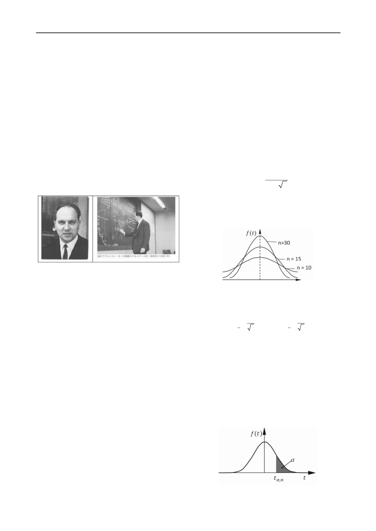
then the distribution of t is the student t distribution for n
degrees of freedom: t(n). The t distribution is more scattered
than the normal distribution of E, depends on the number n of
modulus values collected in each group, and tends towards the
normal distribution when n becomes large (Fig. 2).
Figure 2. The student t distribution
The properties of the student t distribution together with Eq.1
allow us to write:
, 1
, 1
2
2
1
g
g
g
p
g
n
n
P t
t
n
n
(2)
Where t(α/2,n-1) is the value of t for n-1 degrees off freedom
and a value of α/2, α is the area under the t distribution for
values larger than t (Fig. 3). Eq.2 expresses that there is a (1-α)
degree of confidence that the value of μ
p
is between the values
expressed in the parenthesis.
For our example, we need to determine the number n of
modulus values in the group (number of samples to be collected
and tested during the site investigation) which will lead to a
high probability P that the predicted modulus (μ
g
) will be within
a target tolerance ∆ from the true mean modulus of the
population (μ
p
). Therefore we wish to find the value of n which
will satisfy the probability equation:
target
(1 )
(1 )
g
p
g
P
P
(3)
Figure 3. Definition of the parameter α.


