112
Proceedings of the 18
th
International Conference on Soil Mechanics and Geotechnical Engineering, Paris 2013
Proceedings of the 18
th
International Conference on Soil Mechanics and Geotechnical Engineering, Paris 2013
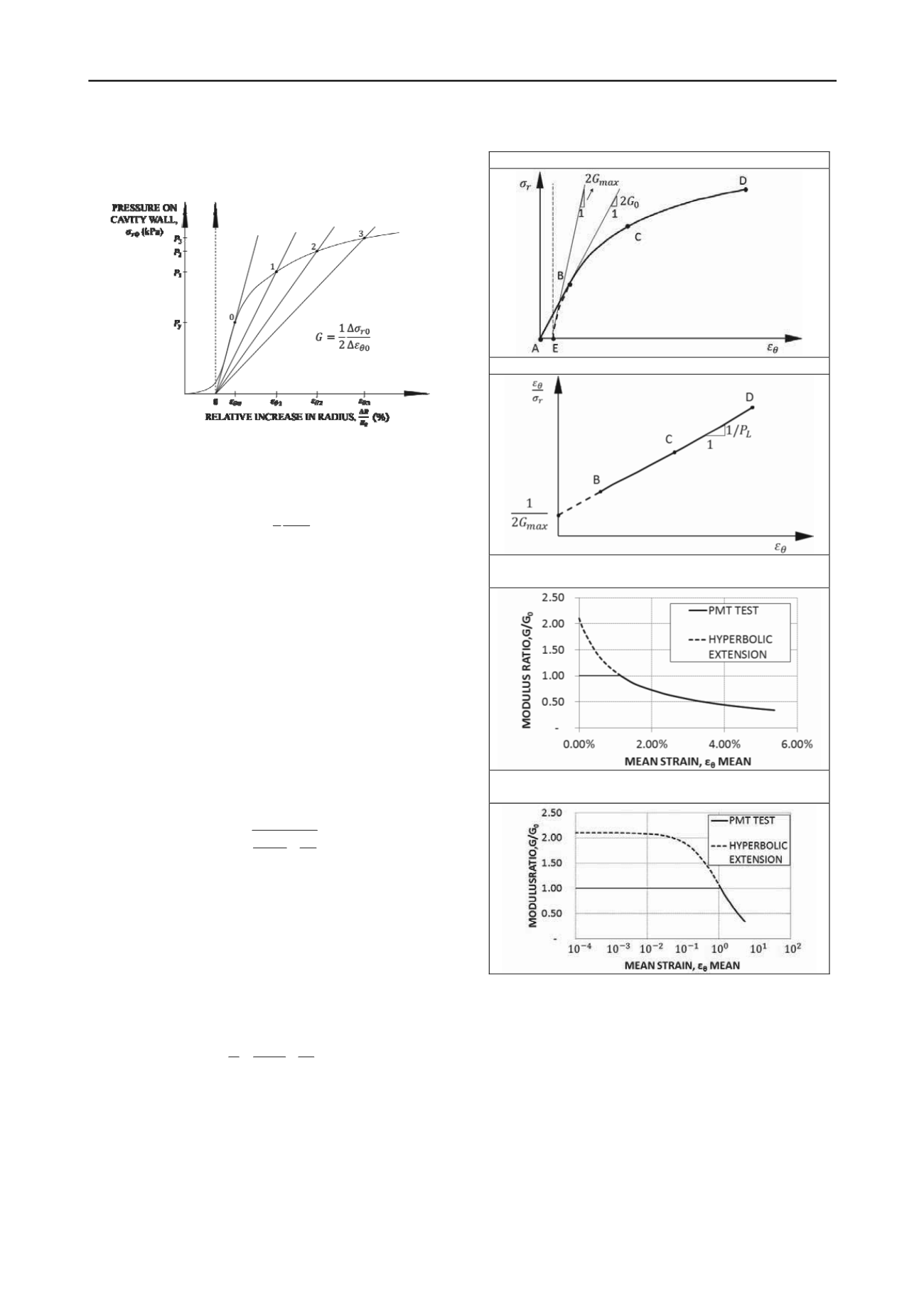
in the PMT) and the strain is the hoop strain ε
θ
(relative increase
in cavity radius). It is therefore possible to define a secant
modulus as a function of strain from the PMT curve (Fig. 9).
Figure 9. PMT stress strain curve and secant modulus
It can be shown in elasticity that the shear modulus is given
by:
1
2
ro
o
G
(34)
If we call G
o
the shear modulus associated with the straight
portion of the curve, we can normalize the modulus at any strain
with respect to G
o
. We calculate the secant shear modulus G
1
,
G
2
, G
3
and so on corresponding to points 1, 2, and 3 on the
pressuremeter curve (Fig. 9). Then we can plot the ratio G
1
/G
o
,
G
2
/G
o
, G
3
/G
o
as a function of the corresponding strain ε
θ1
, ε
θ2
,
ε
θ3
. Note that ε
θ
is the strain at the cavity wall but that the mean
strain ε
θmean
induced in the soil within the zone of influence is
only about 32% of that value (Eq. 33).
The curve linking G/G
o
vs. ε
θmean
is shown on Fig. 10c and
10d. From zero strain to the strain value corresponding to the
end of the straight part of the PMT curve (AB on Fig. 10a), the
G/G
o
vs. ε
θmean
curve is flat on Fig. 10c and 10d because within
that strain range the modulus G is constant and equal to G
o
.
In order to generate the non linear beginning of that curve
(EB on Fig. 10a), it is convenient to assume a hyperbolic model
as proposed by Baud et al. (2013) of the form
max
1
2
L
G p
(35)
This equation defines a hyperbola which describes the PMT
curve with the limit pressure p
L
as the asymptotic value and
2G
max
as the initial tangent modulus. The hyperbolic model has
been shown to be very successful in describing the stress strain
curve of soils (Duncan, Chang, 1970). In Eq. 35, p
L
is known
and all the points on the PMT curve, after excluding the points
on the straight line part, can be used to find the optimum value
of G
max
by best fit regression. This can be done by plotting the
data points as ε/σ vs. ε and fitting a straight line through the data
points (Fig. 10b). Then 1/2G
max
is the ordinate at ε = 0 and 1/p
L
is the slope of the line.
max
1
2
L
G p
(36)
Then Eq. 35 gives the complete curve. This technique was used
at two sites, a stiff clay site near Houston, Texas, and a medium
dense sand site in Corpus Christi, Texas. Example results are
presented in Fig. 11 which shows that the data fits well with a
hyperbolic equation. For these two sites, the average ratio
G
max
/G
o
was 1.75 for the stiff clay and 1.27 for the dense sand.
a. REZEROED PMT CURVE
b. HYPERBOLIC CURVE FITTING
c . NORMALIZED SECANT SHEAR MODULUS VS
STRAIN
d . NORMALIZED SECANT SHEAR MODULUS VS
LOG OF STRAIN
Figure 10. Normalized secant shear modulus vs. strain
Estimates of G
max
were calculated independently by using
correlations proposed by Seed et al. (1986) based on SPT blow
count for sand, Rix and Stokoe (1991) based on CPT point
resistance for sand, and Mayne and Rix (1993) based on CPT
point resistance and void ratio for clays. These estimates of
G
max
were consistently much higher than the values obtained by
the hyperbolic extension of the PMT curve; 25 times larger for
the stiff clay and 44 times larger for the dense sand. This
indicates that this hyperbolic fit to the PMT curve does not lead
to accurate very small strain moduli.


