120
Proceedings of the 18
th
International Conference on Soil Mechanics and Geotechnical Engineering, Paris 2013
Proceedings of the 18
th
International Conference on Soil Mechanics and Geotechnical Engineering, Paris 2013
known and the PMT curves were measured at various depths
within the depth D
v
. An average PMT curve was created within
D
v
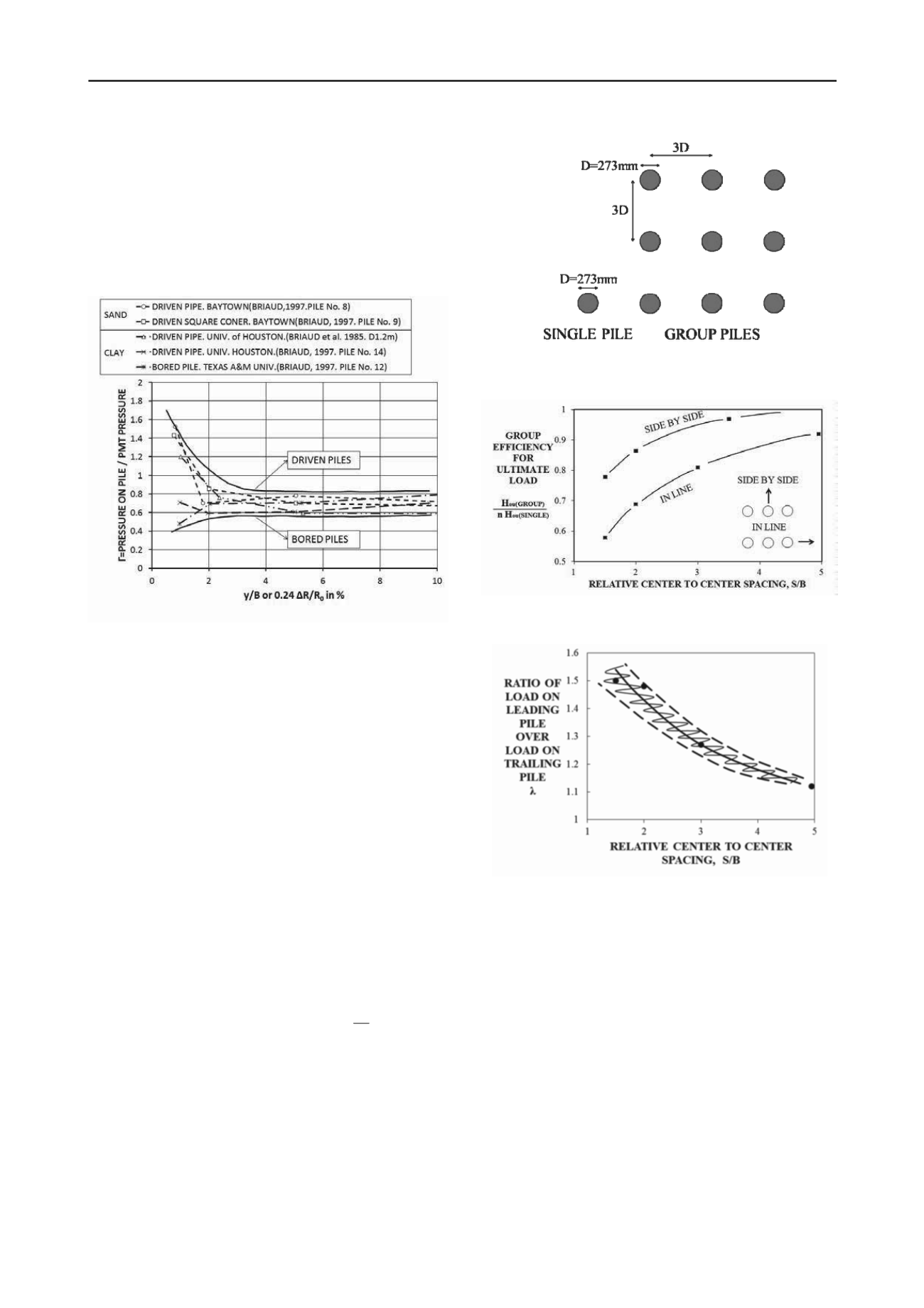
if more than one test was available. The Γ functions obtained
from these load tests and parallel PMT tests are shown in Fig.
22. They have a shape similar to the one for the shallow
foundations but the pile installation seems to make a difference.
The driven piles lead to one class of Γ functions while the bored
pile leads to a lower function. More data would help refine this
first observation.
Figure 22. The Γ functions for transforming the PMT curve into
a horizontal load – displacement curve for a pile.
10.2 Pile group behavior
The behavior of vertically loaded pile groups is often predicted
by making use of an efficiency factor of the form
g v s
Q e nQ
(53)
Where Q
g
is the vertical load on the group, e
v
the efficiency of
the vertically loaded group, n the number of piles in the group,
and Q
s
the vertical load on the single pile for the same
settlement as the pile group. This approach can be extended to
the problem of horizontal loading on a pile group by writing
g h s
H e nH
(54)
Where H
g
is the horizontal load on the group, e
h
the efficiency
of the horizontally loaded group, n the number of piles in the
group, and H
s
the horizontal load on the single pile for the same
horizontal movement as the pile group. Fig. 23 shows the plan
view of a group of horizontally loaded piles.
A distinction is made between the leading piles on the front
row of the group and the trailing piles behind the front row.
Using data by Cox et al. (1983), Briaud (2013) proposed to
extend Eq. 54 to read:
(
)
lp
g
lp lp tp tp s
lp lp tp
s
e
H n e n e H n e n H
(55)
Where n
lp
and n
tp
are the number of leading piles and trailing
piles in the group respectively, e
lp
and e
tp
are the efficiency
factors for the leading pile and trailing pile respectively, and λ is
the ratio of e
lp
over e
tp
. Fig. 24 and 25 give the efficiency factors
as a function of the relative pile spacing based on the data by
Cox et al. (1983).
Figure 23. Plan view of a group of horizontally loaded piles.
Figure 24. Leading pile and trailing pile efficiency factors
Figure 25. Ratio of leading over trailing pile efficiency factor
Eq. 52 was developed based on ultimate load observations at
large horizontal displacements. The use of the same equation for
all range of horizontal movements was investigated by
comparing measured and predicted movements for two major
pile group experiments by Brown and Reese (1985) in stiff clay
and by Morrison and Reese (1986) in medium dense sand. The
plan view of the group is shown in Fig.23. The piles were
0.273m in diameter, 13.1m long steel pipe piles driven in a 3 by
3 group with a spacing of 3 diameter center to center. The group
was built to simulate a rigid cap condition which is most
common. The clay was a stiff clay which had an undrained
shear strength of about 100kPa within the top 3 m from the
ground surface. The sand was a medium dense fine sand with a
CPT point resistance increasing from zero at the ground surface
to 3000 kPa at a depth of 2 m. Fig. 26 presents the result for the
test in clay and Fig. 27 for the test in sand. In each case, the
measured load-displacement curve for the single pile is
presented as well as the measured curve linking the average
load per pile in the group and the group displacement. The


