124
Proceedings of the 18
th
International Conference on Soil Mechanics and Geotechnical Engineering, Paris 2013
Proceedings of the 18
th
International Conference on Soil Mechanics and Geotechnical Engineering, Paris 2013
d. IMPACT TEST: FORCE VS. MOVEMENT
0
200 400 600 800 1000
0
100
200
300
400
500
Static
Experiment
TAMU-POST (Excel)
LS-DYNA
LOAD (kN)
x DISPLACEMENT (mm)
Figure 32. Pick-up truck impact test results
12 LIQUEFACTION CHARTS
Liquefaction charts have been proposed over the years to
predict when coarse grained soils will liquefy. In those charts
(Fig. 33), the vertical axis is the cyclic stress ratio CSR defined
as τ
av
/ σ’
ov
where τ
av
is the average shear stress generated
during the design earthquake and σ’
ov
is the vertical effective
stress at the depth investigated and at the time of the in situ soil
test. On the horizontal axis of the charts is the in situ test
parameter normalized and corrected for the effective stress level
in the soil at the time of the test. There is a chart based on the
normalized SPT blow count N
1-60
(Youd and Idriss, 1997).
There is another chart based on the normalized CPT point
resistance q
c1
(Robertson and Wride, 1998). Using the
correlations in Table 4, it is possible to transform the SPT and
CPT axes into a normalized PMT limit pressure axis as shown
in Fig. 34. The normalized limit pressure p
L1
is
0.5
1
'
a
L
L
ov
p
p p
(63)
Where p
L
is the PMT limit pressure, p
a
is the atmospheric
pressure, and σ’
ov
is the vertical effective stress at the depth of
the PMT test. Note that the data points on the original charts are
not shown on the PMT chart not to give the impression that
measurements have been made to prove the correctness of the
chart. Some degree of confidence can be derived from the fact
that the two charts give reasonably close boundary lines.
Nevertheless, these two charts are very preliminary in nature
and must be verified by case histories.
a. PMT CHART BASED ON CORRELATION WITH
SPT (adapted from Youd and Idriss, 1997)
b. PMT CHART BASED ON CORRELATION WITH
CPT (adapted from Robertson and Wride, 1998)
Figure 33. Preliminary liquefaction charts based on the
pressuremeter limit pressure
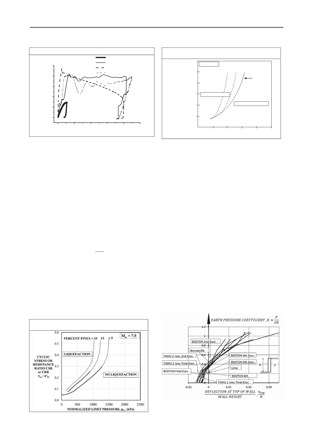
13 ANALOGY BETWEEN PMT CURVE AND EARTH
PRESSURE-DEFLECTION CURVE FOR RETAINING
WALLS
The load settlement curve method for shallow foundations
shows how one can use the PMT curve to predict the load
settlement curve of a shallow foundation. This load settlement
curve method was extended to the case of horizontally loaded
piles. Can a similar idea be extended to the earth pressure versus
deflection curve for retaining walls? One of the issues is that the
PMT is a passive pressure type of loading so the potential for
retaining walls may be stronger on the passive side than on the
active side. Another issue is that the PMT test is a cylindrical
expansion while the retaining wall is a plane strain problem.
Fig. 34 shows the curves generated by Briaud and Kim (1998)
based on several anchored wall case histories. The earth
pressure coefficient K was obtained as the mean pressure p on
the wall divided by the total vertical stress at the bottom of the
wall. The mean pressure p was calculated by dividing the sum
of the lock-off loads of the anchors by the tributary area of wall
retained by the anchors. For each case history the lock off loads
were known and the deflection of the wall was measured. Then
the data was plotted with K on the vertical axis and the
horizontal deflection at the top of the wall divided by the wall
height on the horizontal axis. The shape of the curve is very
similar to the shape of a PMT curve and a transformation
function like the Γ function for the shallow foundation may
exist but this work has not been done.
Figure 34. Earth pressure coefficient vs. wall deflection (after
Briaud, Kim, 1998).


