102
Proceedings of the 18
th
International Conference on Soil Mechanics and Geotechnical Engineering, Paris 2013
Proceedings of the 18
th
International Conference on Soil Mechanics and Geotechnical Engineering, Paris 2013
2
d
op,up
n
n
v
2
1 C sN
D
F
(48)
where N
p
is a bearing factor, s
u,op
is the operative shear strength
at a shear strain rate that reflects the (normal component of)
flow velocity, v
n
, and C
d
is a drag coefficient. The relationship
was calibrated against numerical analysis data (Zakeri 2009),
and yielded drag coefficients in the range 0.6 to1.2 for flow
angles between 30 and 90 º.
The principle behind Equation (48) is that the bearing factor,
N
p,
in common with other bearing factors in geotechnics,
captures the geometry of the failure mechanism, and should be
independent of velocity or soil strength, essentially as specified
in Equation (13) but with adjustment for the relative depth of
the debris flow compared with the pipeline diameter. The effect
of velocity, or shear strain rate, is incorporated into the
operative shear strength, using conventional relationships such
as the Herschel-Bulkley expression in Equation (42), or a
simple power law relationship:
ref
n
ref ,u
ref
ref ,u
op,u
D/ v
s~
s
s
(49)
The relative magnitudes of the two components in Equation
(48) are such that the fluid drag term only becomes significant
once the Johnson number (also referred to as the non-
Newtonian Reynolds number),
v
n
2
/s
u,op
exceeds about 5. The
accuracy of this approach has recently been demonstrated
through experimental work (Sahdi et al. 2013), where a drag
factor of around 1.1 to 1.4 was suggested. Numerical analyses
using the material point method (Ma, private communication)
has confirmed a drag factor close to unity.
For flow parallel to the pipeline, analytical relationships
have been derived for material that follows a power law
function, as in Equation (49) (Einav and Randolph, 2006). The
axial force per unit length, F
a
, is given by
1 12 f
where
D sf F
a
op,ua a
(50)
The value of f
a
lies in the range 1.2 to 1.4 for typical values of
between 0.05 and 0.15.
For the general case of debris flow impacting a pipeline at an
angle
, a failure envelope may be developed to quantify the
interaction between parallel and normal components of force.
Based on the numerical data from Zakeri (2009), a failure
envelope of the form
7.0
90,p
p
1
90,p
p
3
0,a
a
sin
N N
with 1
N
N
f
f
(51)
was found to give a reasonable fit (Randolph and White 2012).
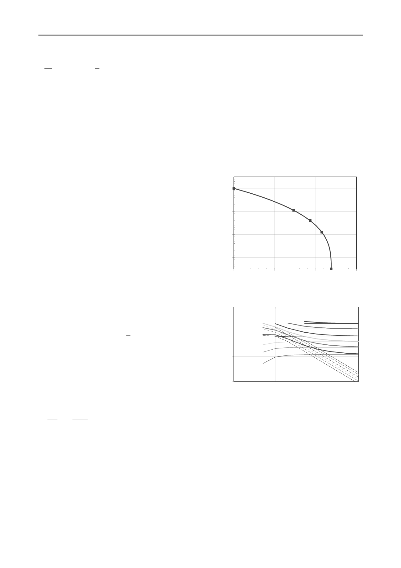
An example failure envelope, taking f
a,0
= 1.4 and N
p,90
= 11.9
as appropriate for a rough pipe, is shown in Figure 27, together
with spot points for flow angles of 0, 30, 45, 60 and 90 º.
Assessment of pipeline response to debris flow impact
requires initial estimation of debris flow velocity, height (which
affects N
p
), relative angle and shear strength at the point of
impact. These are non-trivial quantities to estimate, but may be
gleaned from numerical modelling of landslide runout. The
resulting impact forces and pipeline response may then be
evaluated using the relationships summarised here.
An important consideration is that the normal velocity, v
n
,
used to determine the strain rate (hence operative shear
strength) and the drag force should be the
relative
velocity
between debris flow and pipeline. Initially, as the debris flow
strikes the pipeline, it will carry the pipe with it. Resisting
bending moments and axial tension in the pipeline will develop
quite gradually as the pipeline is deformed. These will slow the
pipeline, relative to the debris flow, until a dynamic equilibrium
is established (Boylan and White 2013).
A single set of results from Randolph et al. (2010) is shown
in Figure 28, for a case where the passive horizontal resistance
of the pipeline outside the slide zone is half the active force, F
n
,
and the passive axial resistance is 25 % of F
n
. The total active
loading, F
n
times the slide zone width B, is normalised by the
pipeline cross-sectional rigidity, EA. The strains in the pipe
become dominated by axial tension as the width of the debris
flow increases; it is evident that relatively low levels of active
loading can cause significant strains, and potentially failure of
the pipeline.
0
0.2
0.4
0.6
0.8
1
1.2
1.4
1.6
0
5
10
15
Axial coefficients, f
a
Normal coefficients, N
p
0
º
30 º
60 º
90 º
45 º
Failure envelope
Relative angle
between debris flow
and pipelines
Figure 27 Failure envelope for varying flow angle relative to pipe axis
(Randolph and White 2012).
0.00001
0.0001
0.001
0.01
10
100
1000
10000
Maximum pipeline strain,
/E
Normalized debris flow width, B/D
Bending
Tension
Combined
F
n
B/EA = 0.001
0.0005
0.0002
0.0001
0.00005
0.00002
Figure 28 Effect of slide loading and width on maximum pipeline strain
(Randolph et al. 2010).
7 CONCLUSIONS
Analysis underpins and enriches design approaches that we use
in day to day practice. Where empirical correlations are still
relied upon, we should strive continuously to understand the
underlying processes and gradually capture them quantitatively
through analysis or synthesis of well-considered numerical
studies. The paper has dipped into a number of different
application areas in offshore geotechnical design, with the aim
throughout being to present simplified outcomes, based on
analysis, that can be applied directly in design. It should be
emphasised, however, that simplifications and idealisations in
analytical solutions are such that final validation and fine-tuning
of a design will often require further input from physical or
numerical modelling of the specific application. Even there
though, analytical solutions should guide the planning of the
more sophisticated investigations.


