767
Technical Committee 103 /
Comité technique 103
Figure 12. Calibration of horizontal soil springs at the north tower by
matching the push-over behaviour in the IBDAS model with the push-
over behaviour in the 2D Plaxis model.
5 RESULTS
Figure 14.
in the brid
tower.
The di
the soil a
parallel w
5.4
Imp
The Mohr-Coulomb material model with
′ =
8 kN/m
3
,
= 78
MPa,
= 0.3
,
= 45°
and
= 15°
is used for the
gravel. The pile is modelled as a rigid body. The load-
displacement behaviour is determined by applying different
vertical loads to the caisson bottom slab and pushing it in
horizontal direction.
The hyperbolic backbone curves with
,
= 30
MPa/m match the results from the 3D finite element model
reasonably well, as shown in Figure 11.
4.4
Horizontal soil springs
The hyperbolic backbone curves of the horizontal soil springs
are calibrated based on a vertical tower foundation load plus a
horizontal force with a lever arm. The lever arm is chosen such
that it represents the average observed lever arm in the seismic
time history analyses with the global model.
A reasonable agreement between the push-over behaviour in
the IBDAS model and the 2D Plaxis model can be achieved
with an initial stiffness
,
= 2.1MPa/m
and a maximum
shear stress
= 0.70 MPa
at the north tower, cf. Figure 12,
and
,
= 0.35MPa/m
and a maximum shear stress
= 0.22 MPa
at the south tower.
4.5
Dashpots
The vertical distributed material and radiation dashpots have
been derived based on linear elastic formulas given in Gazetas
1991 and the spring stiffness according to Section 4.2. The
dashpot coefficients are
= 0.97MPa ∙ s/m ∙ A
at the north
tower and
= 0.74MPa ∙ s/m ∙ A
at the south tower.
Similarly, based on Gazetas 1991 and the spring stiffness
according to Section 4.4, the horizontal distributed radiation
dashpot coefficients are determined as
= 0.24MPa ∙ s/m ∙
A
at the north tower and
= 0.11MPa ∙ s/m ∙ A
at the
south tower.
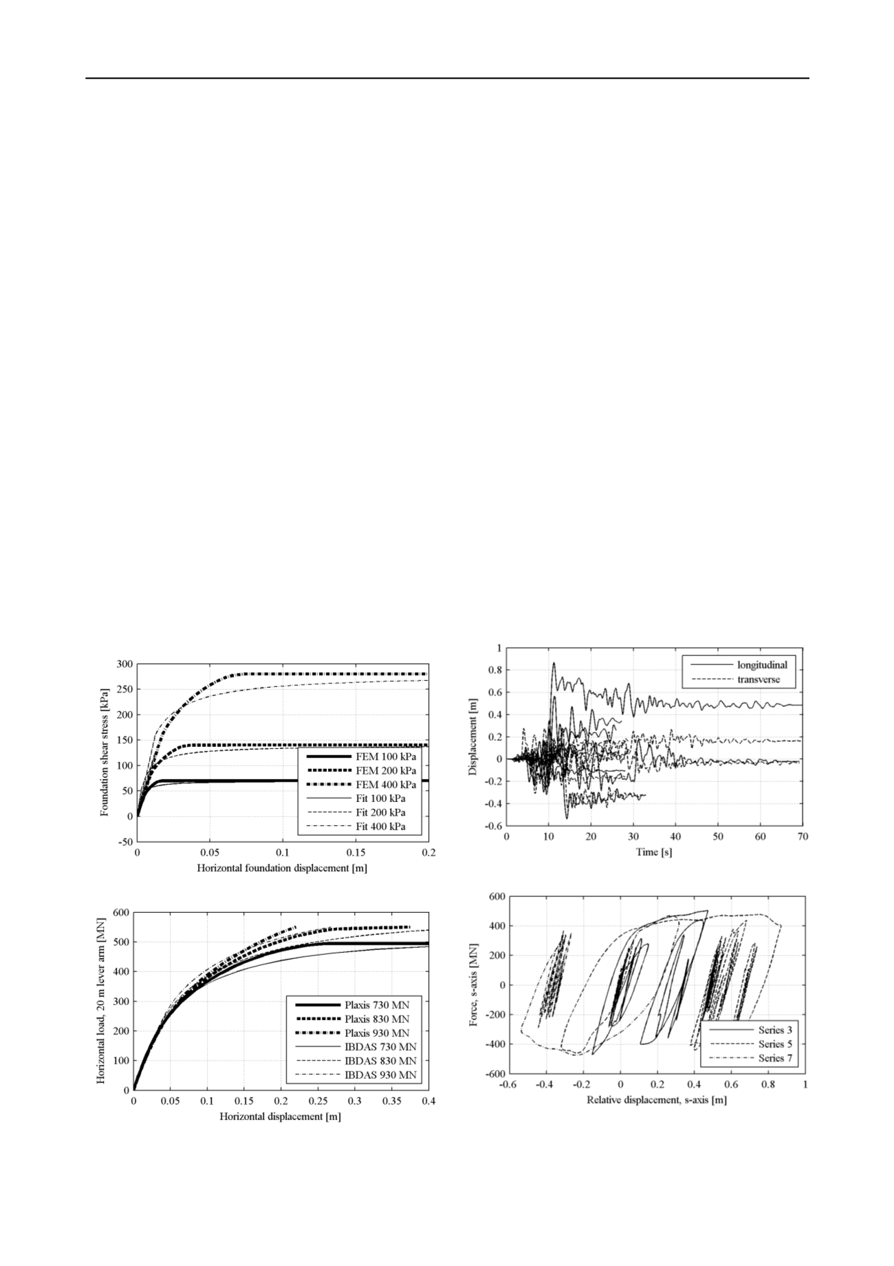
Figure 11. Load-displacement curves from the FE model and fitted
hyperbolic backbone curves.
Figure 12. Calibration of horizontal soil springs at the north tower by
matching the push-over behaviour in the IBDAS model with the push-
over behaviour in the 2D Plaxis model.
5 RESULTS
5.1
Relative displacements
The relative displacement between the centre of the caisson and
the free-field displacements of the soil is exemplified in Figure
13. Irreversible displacements of the caissons are clearly visible.
5.2
Hysteretic behaviour
The intended hysteretic behaviour is indeed produced in the
finite element model, as it can be observed in Figure 14.
5.3
Response in individual springs
While the above curves illustrate the overall behaviour of the
foundations, the response in individual soil and gravel springs
can provide information on the
local
magnitude of displacement
in
-
the interface between soil and structure (gravel springs)
-
the soil volume below the gravel bed (soil springs)
This distribution can be of importance for evaluating how
onerous a plastic deformation is. The gravel spring can be
considered ductile, where plastic deformation typically can be
attributed to sliding in the gravel-foundation interface. In
contrast, plastic deformation in the soil springs must typically
be attributed to incipient yielding in the improved ground, and
its magnitude should therefore be given great consideration.
An example of these displacements is shown in Figures 15
and 16. The spring is located at a foundation corner point, and
the gapping behaviour in the gravel spring can be seen as stress-
free displacements (horizontal parts of the dashed line at
= 0
in Figure 16). Further, it can be observed that at this location,
the majority of the displacements occur in the gravel spring.
Figure 13. Relative displacement for seven NCE time histories, north
tower.
Figure 14. Force vs. relative displacement between foundation and soil
in the bridge longitudinal direction. NCE seismic time histories, north
tower.
The difference in the maximum value of the shear stress in
the soil and gravel springs is due to the radiation dashpot in
parallel with the horizontal soil spring, cf. Figure 5.
5.4
Impact of non-linear effects
The Mohr-Coulomb material model with
′ =
8 kN/m
3
,
= 78
MPa,
= 0.3
,
= 45°
and
= 15°
is used for the
gravel. The pile is modelled as a rigid body. The load-
displacement behaviour is determined by applying different
vertical loads to the caisson bottom slab and pushing it in
horizontal direction.
The hyperbolic backbone curves with
,
= 30
MPa/m match the results from the 3D finite element model
reasonably well, as shown in Figure 11.
4.4
Horizontal soil springs
The hyperbolic backbone curves of the horizontal soil springs
are calibrated based on a vertical tower foundation load plus a
horizontal force with a lever arm. The lever arm is chosen such
that it represents the average observed lever arm in the seismic
time history analyses with the global model.
A reasonable agreement between the push-over behaviour in
the IBDAS model and the 2D Plaxis model can be achieved
with an initial stiffness
,
= 2.1MPa/m
and a maximum
shear stress
= 0.70 MPa
at the north tower, cf. Figure 12,
and
,
= 0.35MPa/m
and a maximum shear stress
= 0.22 MPa
at the south tower.
4.5
Dashpots
The vertical distributed material and radiation dashpots have
been derived based on linear elastic formulas given in Gazetas
1991 and the spring stiffness according to Section 4.2. The
dashpot coefficients are
= 0.97MPa ∙ s/m ∙ A
at the north
tower and
= 0.74MPa ∙ s/m ∙ A
at the south tower.
Similarly, based on Gazetas 1991 and the spring stiffness
according to Section 4.4, the horizontal distributed radiation
dashpot coefficients are determined as
= 0.24MPa ∙ s/m ∙
A
at the north tower and
= 0.11MPa ∙ s/m ∙ A
at the
south tower.
Figure 11. Load-displacement curves from the FE model and fitted
hyperbolic backbone curves.
Figure 12. Calibration of horizontal soil springs at the north tower by
matching the push-over behaviour in the IBDAS model with the push-
over behaviour in the 2D Plaxis model.
5 RESULTS
5.1
Relative displacements
The relative displacement between the centre of the caisson and
the free-field displacements of the soil is exemplified in Figure
13. Irreversible displacements of the caissons are clearly visible.
5.2
Hysteretic behaviour
The intended hysteretic behaviour is indeed produced in the
finite element model, as it can be observed in Figure 14.
5.3
Response in individual springs
While the above curves illustrate the overall behaviour of the
foundations, the response in individual soil and gravel springs
can provide information on the
local
magnitude of displacement
in
-
the interface between soil and structure (gravel springs)
-
the soil volume below the gravel bed (soil springs)
This distribution can be of importance for evaluating how
onerous a plastic deformation is. The gravel spring can be
considered ductile, where plastic deformation typically can be
attributed to sliding in the gravel-foundation interface. In
contrast, plastic deformation in the soil springs must typically
be attributed to incipient yielding in the improved ground, and
its magnitude should therefore be given great consideration.
An example of these displacements is shown in Figures 15
and 16. The spring is located at a foundation corner point, and
the gapping behaviour in the gravel spring can be seen as stress-
free displacements (horizontal parts of the dashed line at
= 0
in Figure 16). Further, it can be observed that at this location,
the majority of the displacements occur in the gravel spring.
Figure 13. Relative displacement for seven NCE time histories, north
tower.
Figure 14. Force vs. relative displacement between foundation and soil
in the bridge longitudinal direction. NCE seismic time histories, north
tower.
The difference in the maximum value of the shear stress in
the soil and gravel springs is due to the radiation dashpot in
parallel with the horizontal soil spring, cf. Figure 5.
5.4
Impact of non-linear effects


