774
Proceedings of the 18
th
International Conference on Soil Mechanics and Geotechnical Engineering, Paris 2013
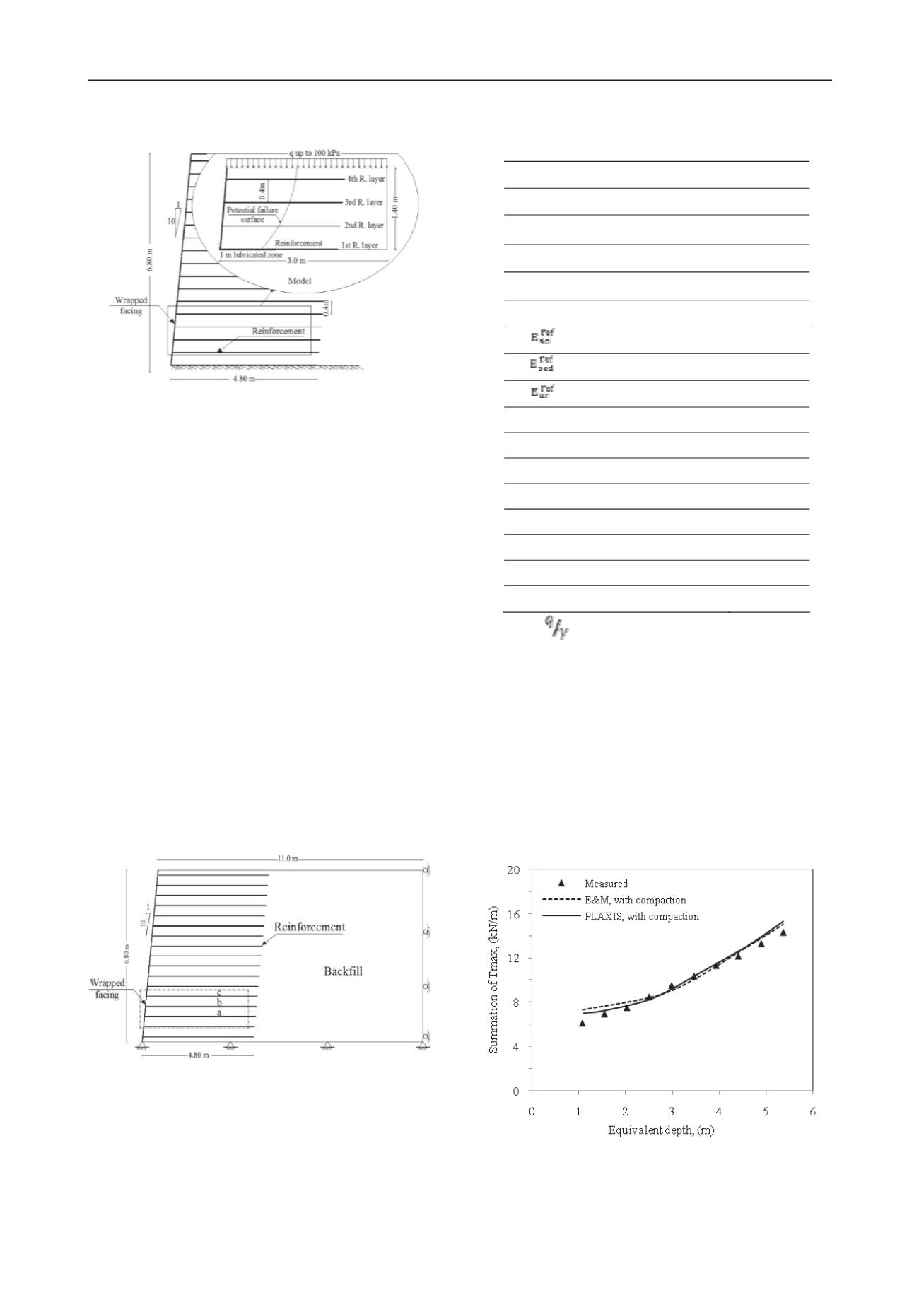
Figure 1. View of prototype and model.
Fig. 2 shows the geometry of the numerical model used in
the performed analyzes. Note that the simulated geometry
represented the prototype. To compare the values determined
with PLAXIS and the measured ones, the summations of the
mobilized maximum tension in the reinforcements “a”, “b”, and
“c” (see Fig. 2), which were representative of the verified values
in the 2
nd
, 3
rd
, and 4
th
reinforcement layers in the physical
model, were used (see Fig. 1). The wall was 6.8 m high and the
length of soil mass assumed in the performed analysis was 11
m. The length and the vertical spacing of reinforcements were
4.8 m and 0.4 m, respectively. The wrapped facing with an
inclination of 6° to the vertical was modeled. In the performed
study, the hardening soil model was applied, which is a
hyperbolic soil model, very similar to the model of Duncan and
Chang (1970). Boundary conditions of the performed numerical
modeling consider horizontal restriction for the right side, and
horizontal and vertical restrictions for the bottom of the wall.
Stage construction was considered; for every 0.2 m of soil
placed, the layer was compacted, until the final wall height was
reached. Compaction was simulated by applying a single load-
unload stress cycle of 63 kPa distribution load at the top and
bottom of each backfill soil layer. This simple approach might
represent the actual multi-cycle load-unload stress path during
compaction (Ehrlich and Mitchell, 1994).Table 1 shows the
input parameters used in this validation. The backfill soil
stiffness and resistance parameters were determined from plane-
strain tests.
Fi
gure 2. Model geometry adopted from prototype.
In Fig. 3, the FEM results are evaluated. This figure shows
the comparison of the determined summation of the maximum
reinforcement tensile stress, T
max
, with those observed from the
physical modeling study, and also the values predicted by the
Ehrlich and Mitchell (1994) method. For details about the
prediction of T
max
by this method, the reader is directed to the
papers by Ehrlich and Mitchell (1994) and Ehrlich et al. (2012).
The equivalent depth of the soil layer (Z
eq
) is defined by:
Table 1. Input parameters for validation analysis.
Parameter
Value
Backfill Soil
Peak plane strain friction angle
(
o
)
50
Cohesion
c
(kPa)
1.0
Dilation angle
Ψ
(
o
)
0.0
Unit weight
γ
(kN/m
3
)
21
(kPa)
42500
(kPa)
31800
(kPa)
127500
Stress dependence exponent
m
0.5
Failure ratio
R
f
0.7
Poisson’s ratio
υ
0.25
Reinforcement
Elastic axial stiffness (kN/m)
600
Face
Elastic axial stiffness (kN/m)
60
Elastic bending stiffness (kNm
2
/m)
1.0
Z
eq
= Z + (1)
where
Z
,
q
, and
γ
are the real depth of the specific layer,
surcharge load value, and soil unit weight, respectively. As
shown, the values measured from the physical model were
properly represented by both the analytical method (Ehrlich and
Mitchell, 1994) and the numerical (PLAXIS) method. However,
for the values of equivalent depth lower than the compaction
influence depth, i.e., Z
eq
< 3 m, the results of the numerical
simulation using PLAXIS was more accurate than the Ehrlich
and Mitchell (1994) method (maximum difference less than
6%). When surcharge load values increased, (i.e., Z
eq
> 3 m),
the measurements, and the values predicted by the Ehrlich and
Mitchell (1994) method and PLAXIS, fully agreed.
Figure 3.Comparison of predicted and measured summations of
maximum tensions along the 2
nd
, 3
rd
, and 4
th
reinforcement layers.


