757
Technical Committee 103 /
Comité technique 103
where u
ey
= yield induced excess pore pressure. The graphical
solution for r
u
’ (Länsivaara 2010) is shown in Figure 3.
0,1
0,12
0,14
0,16
0,18
0,2
0,22
0,24
0,26
18 20 22 24 26 28 30 32 34
friction angle
pore pressure parameter r
u
'
Figure 2. Effective stress pore pressure parameter r
u
’ as function of
friction angle (Länsivaara 2010). The solution is valid for normally
consolidated (K
0
) clays.
This simple method is strictly valid only for active loading, and
in the passive part of the failure envelope the pore pressure
increase would be higher. However, as discussed by Länsivaara
(2010) this error is compensated by the fact that next to the
embankment the soil is at least slightly overconsolidated, which
in turn leads to proportionally lower excess pore pressure.
2.3
Method 2: MUESA
The calculation method “MUESA” (Modified Undrained
Effective Stress Analysis) is partly derived from the method
“UESA” proposed by Svanø (1981). MUESA accounts for
anisotropy, non-triaxial stress states and overconsolidation
In MUESA the amount of excess pore pressure is calculated
based on stress changes in relation to the initial stress state
(before the start of undrained loading). Excess pore pressure Δu
is
d as
expresse :
'
p
p
u
(3)
For a given slip surface, an initial stress state along a slip
surface is calculated assuming K
0
-conditions. This assumption
is not very accurate for slopes but is reasonably valid for
embankments on nearly horizontal soil. The initial stress state is
defined as the state before undrained loading, such as a traffic
embankment without external loading. The embankment with
traffic load applied would then be the design stress state.
An initial assumption for the pore pressure (e.g. ground
water + excess pore pressure) acting on the bottom of each slice
is made. The limit equilibrium is then calculated in regular
fashion (with the loading in place), using this initial pore
pressure assumption. The desired LE method (e.g. Morgenstern-
Price, Janbu’s simplified etc.) can be used. The stress state (σ’
n
,
τ) resulting from the equilibrium is used to calculate the next
assumption for Δu. The process continues iteratively until pore
pressure converges. The value of the initial assumption (within
realism) has no effect on the final result but good assumptions
lead to fast convergence.
To calculate excess pore pressure its two components Δp and
Δp’ need to be calculated. The component Δp can be calculated
by using basic principles of continuum mechanics and the
assumption of the Mohr-Coulomb failure criterion. The two
compared stress points are the initial total mean stress p
0
and
either mobilized or failure total mean stress (p
mob
or p
f
).
A three-dimensional stress space (with three principal
stresses) is used to determine Δp so that non-triaxial stress states
can also be considered (p = p(σ
1
, σ
2
, σ
3
)). The principal stresses
are easily derived using basic continuum mechanics.
The effective stress component Δp’ is derived from the yield
surface formulation of the constitutive soil model S-CLAY1
(Wheeler et al 2003). S-CLAY1 is in good agreement with tests
done on soft, lightly overconsolidated clays. The only
parameters needed to define the initial yield surface are the
friction angle φ’ and the vertical consolidation pressure σ’
c
.
To obtain Δp’ the effective mean stress at failure p’
f
needs to
be calculated. In the current formulation of MUESA it is
assumed that the stress path follows the initial yield surface in
the normally consolidated state (no volumetric hardening), and
the stress path terminates at the intersection of the yield surface
and the failure line. The assumption of no volumetric hardening
can be regarded as the absolute maximum for the amount of
excess pore pressure and minimum of shear strength and the
calculation is thus on the safe side. The effective mean stress at
failure p’
f
is solved as the intersection of the S-CLAY1 yield
surface and the Drucker–Prager failure surface in the principal
stress space (σ
1
, σ
2
, σ
3
).
In MUESA the use of failure pore pressure is considered as
described in Section 2.1. The use of failure pore pressure is
fairly simple as only the initial and failure stress states need to
be considered, and the actual stress path in between can be
disregarded. The method seems to be most sensitive to
assumptions regarding anisotropy, especially in the passive end
of the slip surface. Hardening will be implemented in the future.
3
CALCULATION EXAMPLE
A calculation example is a test embankment from Salo, Finland,
where a full-scale railway embankment failure experiment was
carried out in 2009 (Lehtonen 2011). An embankment on
sensitive clay soil was quickly brought to failure, simulating a
very heavy train coming to a standstill. Extensive pore pressure
measurements were continuously conducted.
Table 1. Soil properties in the example.
Soil
layers
γ [kN/
m
3
]
φ'
[°]
c'
[kPa]
s
u
[kPa]
ds
u
[kPa/m
]
POP
[kPa]
r
u
'
Emb.
20 38 0
Sand fill
19 35 0
Dry crust
17
30
Clay
15 25 0
12
1.5
20
0.2
The soil conditions and calculation parameters are give in Table
1. A small embankment is loaded with a 2.5 m wide rain load.
The subsoil consists of a fill layer of sand, dry crust and a soft,
slightly overconsolidated clay layer (POP = 20 kPa). Under the
soft clay there are layers of clayey silt and moraine, but these
are disregarded here as the slip surface is not located in them.
Ground water level is near the bottom of the dry crust.
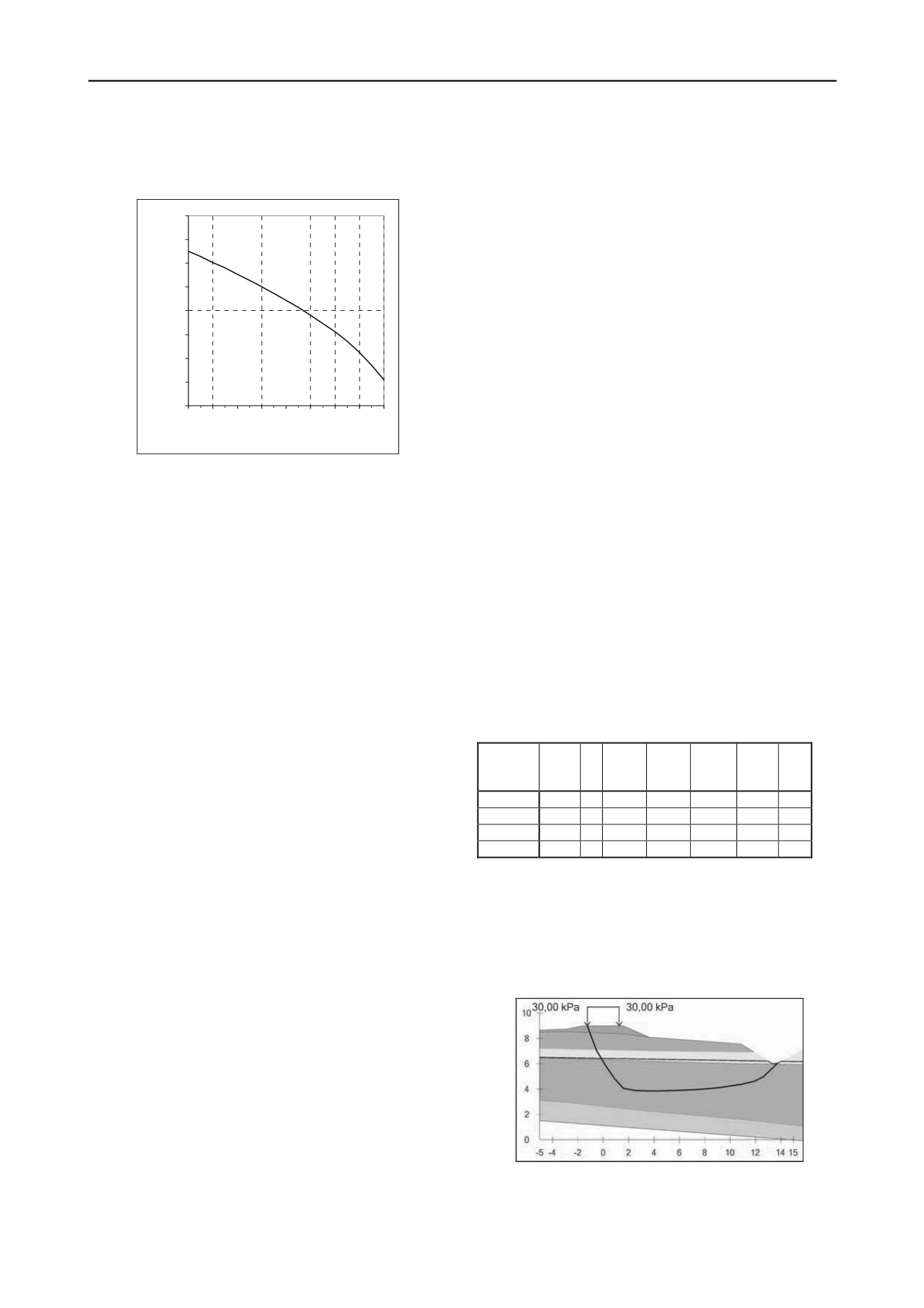
Figure 3. Soil geometry and slip surface used in the example. Soil layers
from top down are embankment, sand fill, dry crust, clay and clayey silt.


