752
Proceedings of the 18
th
International Conference on Soil Mechanics and Geotechnical Engineering, Paris 2013
order to measure the bending moment of the pile during
vibration. The maximum bending moment of the pile was
calculated, using the following equation.
(1)
where,
σ
L
and
σ
R
are the normal stresses at the left and right
outermost pile mesh integration points, respectively; y is the
distance between the integration points and the central axis; and,
I is the the moment of inertia of the pile.
Table 1 shows the test programs. All values are given in
prototype dimensions, which are converted according to scaling
laws for centrifuge testing (Taylor 1995, Iai et al. 2005) As
shown in Table 1, tests were performed under various input
frequency and acceleration conditions, using 12 sine waves and
10 seismic waves. Three different pile diameters were used for
the tests. Calibration was performed after the numerical
modeling, which was carried out for the centrifuge test using the
pile with the largest diameter of 2.5cm and thickness of 0.1cm.
The same procedure was repeated for a pile with a diameter of
1.8cm and thickness of 0.1cm, and the suggested method of
numerical modeling was validated by comparing the results.
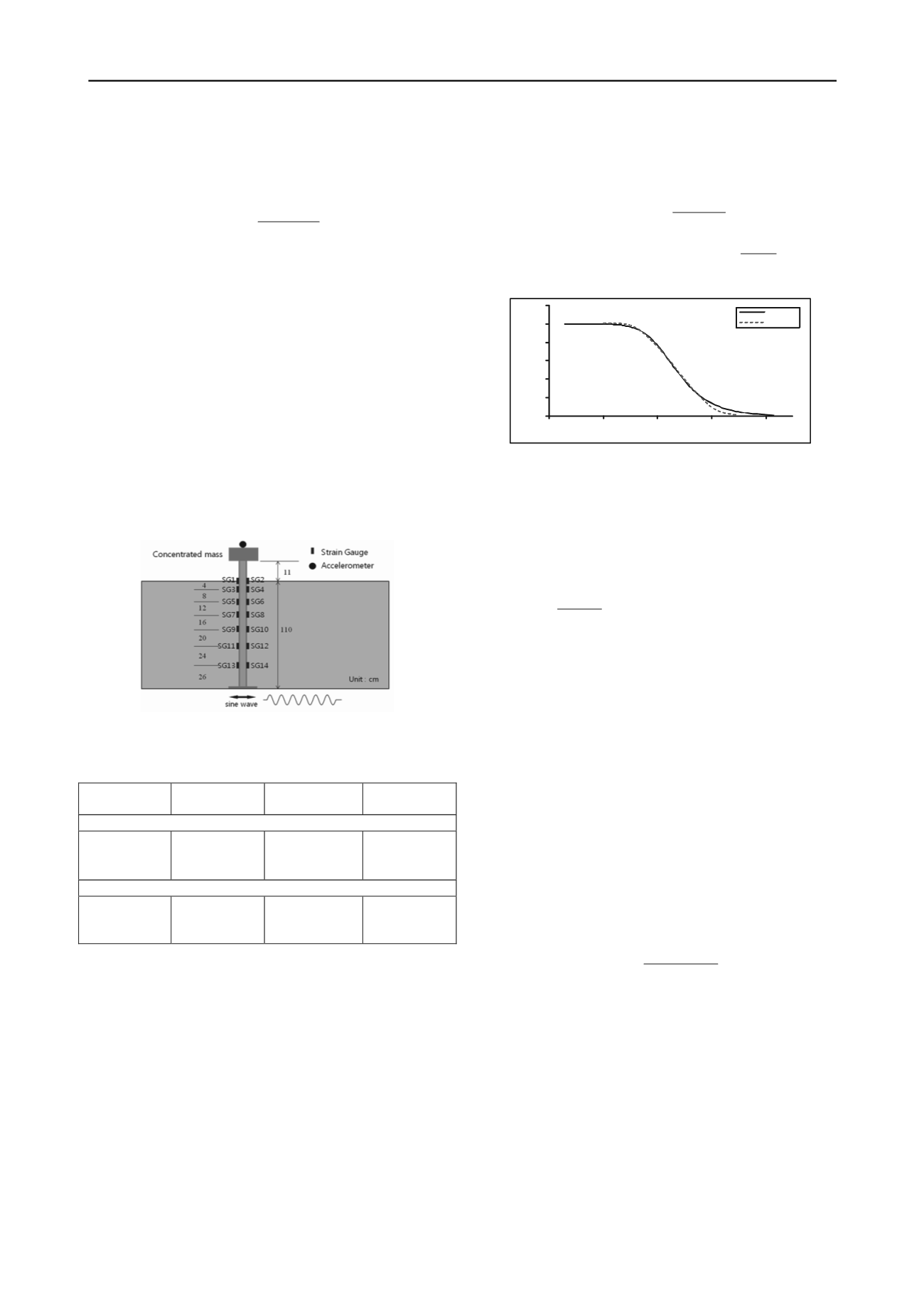
Fig. 1 Layout and Instrumentation
Table 1. Test program
Case
Input motion
Base input
frequency(Hz)
Amplitude of
base input(g)
(a) Sinusoidal wave
a1
a2
a3
-
-
-
1
2
3
0.05, 0.13,
0.25, 0.45
(b) Real earthquake
b1
b2
Ofunato
Nisqually
-
0.06, 0.13,
0.25, 0.36,
0.51
3 3D FINITE DIFFERENCE ANALYSIS
3.1 Soil model
The soil model adopted in this study mainly consists of two
parts, which are the constitutive model and the damping model.
During a strong earthquake, soils show nonlinear plastic
behavior, while large displacements take place. In order to
simulate this type of behavior, the Mohr-Coulomb elastoplastic
model was used as the constitutive model. The nonlinear
behavior of soils was simulated by applying a hysteretic
damping model. As shown in Eq. (2), in the hysteretic damping
model, the tangential shear modulus is represented as a function
of shear strain (Itasca Consulting Group 2006). L1 and L2 of
Eq. (2) represent the decrease rate and decrease starting point of
G/G
max
of the G/G
max
-γ curve, respectively. In this study, the
G/G
max
-γ curve of Jumoonjin sand is obtained by triaxial
compression tests and resonant column tests. L1 and L2 were
determined as 0.5 and 3.65, respectively, by parametric analysis,
and used to calibrate the G/G
max
-γ curve of the numerical model
(Fig. 2)
(2)
Where M
t
is the tangential shear modulus, , L=log
10
γ,
L
1
&L
2
= Coefficient; and γ = is shear strain,
�
Fig. 2 Calibration of G/G
max
(Jumoonjin Sand)
The maximum shear modulus of soils depends on the
confining stresses according to depth (Hardin et al. 1978), and
for this study, the calculation of the maximum shear modulus of
soils was made using Eq. (3). The coefficients A and n were
determined by prior test results (Yang 2009).
(3)
where, , e is the void ratio, is the average
principal stress,P
a
is the atmosphere pressure, and coefficients A
and n are 247.73 and 0.567, respectively.
3.2 Interface model
The interface between pile foundation and surrounding soil
undergoes slippage and separation during strong earthquake
motions. The interface model should consider this kind of
phenomena accordingly. For this study, an interface model that
can simulate the soil-pile separation, of slippage in the normal
and shear directions, was adopted. The applied interface model
uses normal and shear stiffness of the interface, in order to
estimate the spring constant, and the constant is represented as
Eq. (4) (Itasca Consulting Group 2006). The shear modulus
used in Eq. (4) considers the nonlinear behavior of soil, as
represented in 3.1. Therefore, the nonlinear behavior is also
considered in the interface model. Parametric study on the
stiffness showed that the numerical modeling results and test
results were most similar when the shear stiffness and normal
stiffness were identical in value; therefore identical values were
applied (k
n
=k
s
=1.51
×
10
10
N/m):
(4)
where K and G are the bulk and shear modulus of the soil zone,
respectively; and
Δ
z
min
is the smallest dimension of an
adjoining zone in the normal direction.
3.3 Boundary condition
The most important aspect of boundary conditions for
numerical modeling of pile foundations is the simulation of
semi-infinite boundary conditions. When the proper boundary
conditions are not applied, the input motion generates a
reflected wave, resulting in an inaccurate simulation of actual
motion. In addition, if modeling is done with an endless number
of meshes, analysis time greatly increases, resulting in difficulty
for numerical analysis for various conditions, and decrease of
analysis efficiency. Therefore, in order to overcome the
problems stated above, simplified continuum modeling was
adopted (Kim et al. 2012). Fig. 3 shows a layout of the
2
2 1
6 (1
(3 2 )
t
s s
10
) log
s
s
e
L L
M
max
(
)
L
R
M
I
y
2
2
1
L L
s
L L
0
0.2
0.4
0.6
0.8
1
1.2
0.000001 0.0001
0.01
1
100
G
/G
m
ax
��� �
L1=0.5,L2=-3.65
Measured
Calculated
1
'
max
( )(
)
( )
k
n
n
a
m
F e OCR P
G A
2
1
F e
e
'
m
( )
0.3 0.7
min
(4 / 3)
max[
]
n
K G
k
z


