745
Technical Committee 103 /
Comité technique 103
Proceedings of the 18
th
International Conference on Soil Mechanics and Geotechnical Engineering, Paris 2013
3
where
v
is the velocity field,
p
is the density field,
ρ
is the
pressure field, ”
g
” is gravity, and
µ
is the viscosity of the
fluid. Fluid implementation in this research was primarily based
on Muller et al. (2003) but has been expanded to use a novel
grid-based data structure and traversal ordering that allows the
system to be computed more efficiently and to be spread across
more CPU Cores than was previously possible. To model the
soil a set of statically placed erodible particles was used as
introduced by Kristof et al. (2009) and Muller et al. (2003).
Three types of particles were used in this simulation; soil
particles, boundary particles (soil particles near a water
particle), and water particles. The method introduced by Briaud
et al. (2008) was used to model the transfer of mass from
boundary particles into water particles based on the shear stress
between the water and soil.
= ∑
(
−
)
(3)
where
K
is the shear stress constant,
n
is the flow behavior
index,
v
rel
is the velocity relative to the solid surface,
l
is the
distance between the fluid and boundary particle,
K
e
is the
erosion strength,
τ
c
is the critical shear stress,
M
b
is the mass of
a boundary particle, and j is a particle within the smoothing
radius.
The model presented by Toon et al. (2008) was used in the
next step of simulation, after modeling water that permeates into
the soil. To do this, the properties porosity and permeability
were added to all of the soil particles in the system. These were
used to model the capillary pressure gradient (Eq. 4), which
gives rise to the Darcy flux (Eq. 5). The fluid mass is then
integrated using explicit Euler integration.
∇
= ∑
∇
−
, ℎ
,
=
(1 −
)
(4)
= ∑
.
∥
∥
(
−
, ℎ
)
(5)
Where
k
c
and 0<
α
<1 control the strength of the potential,
m
pj
is the fluid mass of s dirt particle,
K
is the permeability, and
β
>0
controls flow.
To determine the proper
α
and
β
, a physical permeability test
was performed using a soil mixture whose permeability and
porosity properties are used in the computer simulation (Fig. 3).
Figure 3. Physical saturation tests using soil and clay mixture
After the physical test, 3 soil samples were taken from the
top, middle and bottom of the oil cylinder to gather saturation
statistics. Then 103 computer simulations were executed using
different alpha and beta values to do a statistical analysis of the
impact of each variable on the saturation simulation result at the
given sampling heights. The alpha and beta values acquired
from the analysis above produced the following result (Fig. 4)
in which the time that the wet line took to reach the bottom and
the saturation values at all sampling heights agreed with what
the physical test demonstrated.
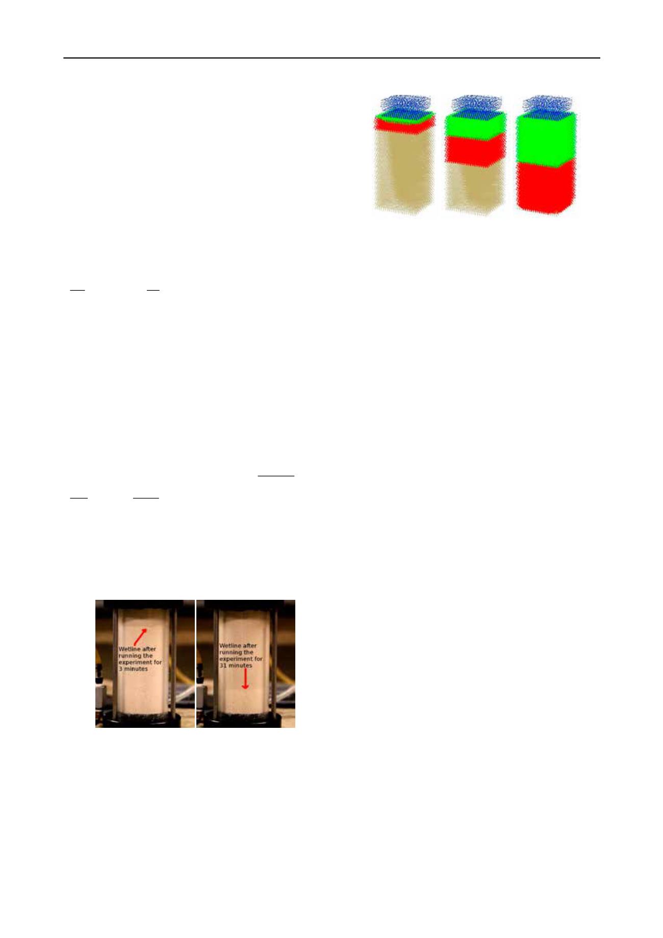
Figure 4. Permeability simulation result produced using proper
α
and
β
values matched physical test result: particles were marked
blue if above 78% saturated (top soil sample saturation), green if
above62% saturated (middle soil sample saturation)and red if
above 32% saturated(bottom soil sample saturation)
Levee erosion was simulated, taking permeability into
account. For each of the simulations approximately 450,000
water and 2,500,000 soil particles were introduced (Chen et al.,
2011). The erosion rate in the simulation, “Z”, (mm/hr) is
modeled by using Eq. 6:
Z=
0
ℎ ≤
× + 0.1 ℎ >
(6)
where
τ
is the hydraulic shear stress (Pa) and
τ
c
is the critical
shear stress. Since the values of
a
and
τ
c
are different for
different materials, their values have to be determined for each
material used in physical experiments. In the authors’ previous
experiments, pure sand and sand-clay mixtures (85% sand and
15% clay) have been used. In previous simulations, the value
for
a
was estimated to be 187 and 93 for pure sand and sand-
clay mixtures respectively, and the value for
τ
c
was estimated to
be 2.0 and 3.0. A series of simulations on those two materials
have been run, as well as some imaginary materials whose
erodibility lies between the erodibility of those two materials
(Chen et al., 2010). In order to determine the values of the
parameters for the material used in the current experiments, a
comparison between the results of previous simulations and the
results of current physical experiments have been done.
Water flow rate, geometry of the levee surface, and
erodibility of the soil were identified as three major components
in the formation of channels during erosion simulation. A total
of 27 computer simulations have been run, one for each possible
combination of three different flow rates, levee down-slope
angles, and erodibility values. For flow rates, values of 8, 11,
and 14 mL/s, were chosen. For erodibility values, 137, 159, and
187 alpha-values, representing the range from sand-clay mixture
made up of approximately 10% clay to pure sand were chosen.
Finally, for levee slope, dry-side slopes of 4:1, 5:1, and 6:1,
typical ranges found in real levee design were chosen. For each
simulation result, the time to breach was visually determined,
and has been identified by the Dam-Break Flood Forecasting
Model.
3 CONCLUSIONS
Times to breach statistics were observed to be based
primarily on the flow rate of the water rushing over the levee.
This appears logical, as a higher velocity implies more shear
stress, and more opportunity to surpass the soil's critical shear
stress and cause erosion. Secondarily, soil erodibility impacted
the level of erosion as well. Within a single flow rate's time set,
highly erodible soil failed first. The slope of the levee geometry
had minimal impact on times to breach, an observation that is
somewhat surprising considering how important levee slope is
in the design of levees, as it has an impact on levee seepage and
levee stability. However, at present our simulation does not


