 
          2967
        
        
          Technical Committee 214 /


            Comité technique 214


            Proceedings of the 18


            th


            International Conference on Soil Mechanics and Geotechnical Engineering, Paris 2013


          2.2


            The influences of the variables on the assessments of U


          The influences of the variables
        
        
          and
        
        
          (Eq. 2) are shown vs.
        
        
          assessed values of
        
        
          in Figure 3 for
        
        
          1.6 metres. The
        
        
          appearance is similar for the other two values of
        
        
          . In models I,
        
        
          II, IV, V and VI, the influences of the other variables were
        
        
          <0.045 for all values on
        
        
          . However, formodel III, the
        
        
          influences of
        
        
          ⁄
        
        
          and
        
        
          ⁄
        
        
          were equal to that of
        
        
          , so that
        
        
          the curves for


            p/


            i


          and


            Cc/Ck


          coincide with the curve for


          (the short-dashed curve). Model I was excluded from this
        
        
          figure, as
        
        
          was equal to 1 for all values of
        
        
          . In the figure, it
        
        
          can be seen that
        
        
          0.8 for
        
        
          0.8, whereafter
        
        
          decreases
        
        
          rapidly and


          (and in case III also


            p/


            i


          and


            Cc/Ck


          ) become
        
        
          progressively more influential.
        
        
          2.3


            The


          variables’


            contribution to


          In Figure 4, the relative influences of the four variables treated
        
        
          stochastically on
        
        
          are shown for
        
        
          1.6 metres. The
        
        
          appearance is similar for the other two values of
        
        
          . It can be
        
        
          seen that
        
        
          contributes more than 50% to
        
        
          in all the
        
        
          analyses, that
        
        
          accounts for most of the remainder and
        
        
          that the contributions from
        
        
          and
        
        
          ⁄
        
        
          are smaller.
        
        
          3 DISCUSSION
        
        
          3.1


            Values on the variables


          The values assigned to the variables in the analyses were chosen
        
        
          by the present authors based on suggestions in the literature and
        
        
          are considered to be representative for soft clays. In the
        
        
          framework of this study (results not presented),
        
        
          for the
        
        
          variables were varied within reasonable ranges one at a time
        
        
          rendering a similar appearance in the results to that presented.
        
        
          Other combinations of the variables might render results that
        
        
          deviate from the results presented here, but it is the authors
        
        
          ’
        
        
          belief that the appearance of the results is typical for most cases.
        
        
          3.2


            The assessed U and the influences of the variables


          As seen in Figure 2, model I followed by model II were the
        
        
          most conservative, predicting the slowest consolidation rate.
        
        
          Comparing the formulations for
        
        
          in model II with those in
        
        
          models IV-VI (Figure 1b and Table 1), this is obvious since
        
        
          model II assigns a constant value of
        
        
          over
        
        
          whereas
        
        
          is
        
        
          successively increased in the other three models. In this context,
        
        
          it should be noted that model III gives lower values of
        
        
          than
        
        
          model II at corresponding
        
        
          for
        
        
          ⁄
        
        
          1 (0.75 in this study).
        
        
          The finding that model I was the most conservative emphasises
        
        
          the relative importance of
        
        
          compared to the modelling of the
        
        
          smear zone. Model I does not take the smear zone into account
        
        
          but adopts
        
        
          instead of
        
        
          (
        
        
          was assumed to be 1.5 times less
        
        
          than
        
        
          in this study). The relative importance of
        
        
          is also
        
        
          shown in Figure 3 where
        
        
          predominates in the assessment of
        
        
          for all but the last parts of the consolidation sequences.
        
        
          The significance of (re)consolidation effects and the
        
        
          associated decrease in
        
        
          (incorporated in model III) is
        
        
          confirmed by the results of laboratory oedometer tests presented
        
        
          by Indraratna and Redana (1998), Sharma and Xiao (2000) and
        
        
          Sathananthan and Indraratna (2006). The results presented in
        
        
          their studies suggest that the resulting decrease in void ratio
        
        
          when the consolidation stresses are increased by 25-50 kPa lead
        
        
          to a more pronounced decrease in
        
        
          than the disturbance
        
        
          induced by the installation process. Hence, in most cases it is
        
        
          more important to consider the change in
        
        
          that occurs due to
        
        
          the decrease in void ratio during consolidation than the
        
        
          disturbance effects.
        
        
          3.3


            The uncertainty in U


          To reduce the uncertainty in the assessment of
        
        
          via any of the
        
        
          investigated models, it is obvious that attention should be
        
        
          directed primarily towards
        
        
          , since the uncertainty in
        
        
          is
        
        
          dependent on
        
        
          via
        
        
          ⁄
        
        
          , and
        
        
          secondarily towards
        
        
          (Figure 4). Hence, site investigations
        
        
          intended for the design of PVDs should focus on reducing the
        
        
          level of uncertainty in
        
        
          and possibly the degree of disturbance
        
        
          in the smear zone (i.e.
        
        
          ).
        
        
          In ordinary engineering projects involving clay, investigations
        
        
          of
        
        
          (e.g. via oedometer tests) are far more frequent than
        
        
          investigations of
        
        
          and it might therefore be worth considering
        
        
          model I. However, if model I is used for design purposes, care
        
        
          must be taken as
        
        
          is used instead of
        
        
          Table 2. Values assigned to the variables in the analyses,
        
        
          is the
        
        
          average value and
        
        
          is the coefficient of variation
        
        
          Variable


            Comment


          5x10
        
        
          -8
        
        
          m
        
        
          2
        
        
          /s
        
        
          A
        
        
          0.35
        
        
          considered
        
        
          representative for soft
        
        
          clays and
        
        
          chosen
        
        
          based on Lumb (1974)
        
        
          0.066
        
        
          m
        
        
          B
        
        
          Det.
        
        
          Rectangular PVD
        
        
          0.003 m x 0.1 m
        
        
          ⁄
        
        
          1.7
        
        
          B
        
        
          Det.
        
        
          Rectangular mandrel
        
        
          0.06 m x 0.12 m
        
        
          ⁄
        
        
          4.7
        
        
          0.34
        
        
          C
        
        
          8
        
        
          0.34
        
        
          ⁄
        
        
          ⁄
        
        
          1.6
        
        
          0.34
        
        
          C
        
        
          ⁄
        
        
          2
        
        
          Det.
        
        
          Arbitrary chosen
        
        
          ⁄
        
        
          0.75
        
        
          0.34
        
        
          D
        
        
          arbitrary chosen
        
        
          2
        
        
          Det.
        
        
          C
        
        
          A


            5x10


            -8


            /1.5=3.3x10


            -8


            m


            2


            /s for model I


          B


            Equivalent diameter evaluated as proposed by Hansbo (1979)


          C


            and


            evaluated from the cited laboratory tests


          D
        
        
          √


            where


            0.3 (Lumb 1974)


            and


            0.15 (from compilation in Müller and Larsson 2012)
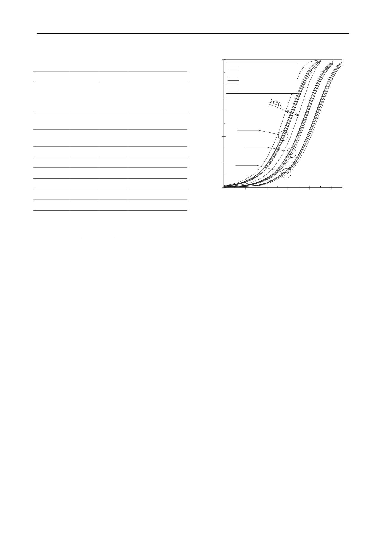


          Figure 2.
        
        
          assessed via the six models for different values of
        
        
          .
        
        
          0
        
        
          0.2
        
        
          0.4
        
        
          0.6
        
        
          0.8
        
        
          1
        
        
          1
        
        
          4
        
        
          16
        
        
          64 256 1024
        
        
          U
        
        
          (-)
        
        
          t
        
        
          (days)


            d


          = 1.1 m


            d


          = 2.1 m


            d


          = 1.6 m


            Kjellman (1949), I


            Hansbo (1979), II


            Indraratna et al. (2005), III


            Walker & Indraratna (2006), IV


            Basu et al. (2006)-b, V


            Basu et al. (2006)-d, VI