 
          2966
        
        
          Proceedings of the 18
        
        
          th
        
        
          International Conference on Soil Mechanics and Geotechnical Engineering, Paris 2013


            Proceedings of the 18


            th


            International Conference on Soil Mechanics and Geotechnical Engineering, Paris 2013


          compression modulus and
        
        
          is the unit weight of water),
        
        
          is
        
        
          the consolidation time,
        
        
          is the diameter of the assumed unit
        
        
          cell dewatered by a single drain (cf. Figure 1) and the
        
        
          expression
        
        
          is dependent on the model.
        
        
          1 METHODS
        
        
          The characteristics and formulations of the expression
        
        
          in the
        
        
          six investigated models are presented in Table 1 and Figure 1b.
        
        
          Denoting the variables in Eq. 1 and in the formulations of
        
        
          (i.e.
        
        
          ⁄
        
        
          ⁄
        
        
          ) as
        
        
          , the partial
        
        
          derivative of
        
        
          with respect to the variable
        
        
          , i.e.
        
        
          ⁄
        
        
          , can
        
        
          be obtained and the influence of each variable on
        
        
          can be
        
        
          assessed:
        
        
          ⁄
        
        
          √∑ (
        
        
          ⁄ )
        
        
          (2)
        
        
          This was done for all of the aforementioned models, assigning
        
        
          (           )
        
        
          metres and for values of
        
        
          resulting in
        
        
          assessments of
        
        
          ranging from 0 to 1. In addition, the
        
        
          uncertainties in the assessments of
        
        
          (expressed as the variance,
        
        
          ) were evaluated. In these analyses, the variables
        
        
          ,
        
        
          ,
        
        
          and
        
        
          ⁄
        
        
          were treated stochastically, while the other variables
        
        
          were assumed to be deterministic, and the variances in the four
        
        
          variables were propagated through Eq. 1 via second order
        
        
          Taylor series approximations (e.g. Fenton and Griffiths, 2008
        
        
          pp. 30-31). The contribution to
        
        
          from each variable was
        
        
          then assessed as (e.g. Christian et al. 1994):
        
        
          (
        
        
          ⁄ )
        
        
          ∑ [(
        
        
          ⁄ )
        
        
          ]
        
        
          (3)
        
        
          Values assigned to the variables adopted in the analyses are
        
        
          presented in Table 2.
        
        
          2 RESULTS
        
        
          2.1


            Assessments of U from the six models


          In Figure 2, the degrees of consolidation
        
        
          assessed from the
        
        
          six models are presented as a function of
        
        
          for the three values
        
        
          of
        
        
          . In the figure, a span representing two standard deviations
        
        
          (SD), i.e.
        
        
          √
        
        
          , is presented for
        
        
          1.1 m. The
        
        
          appearance is similar for the other two values of
        
        
          . The curves
        
        
          plot at a close distance and well within the span of 2xSD for the
        
        
          respective values of
        
        
          , i.e the uncertainties in the variables had
        
        
          a greater impact on the assessed value of
        
        
          than the choice of
        
        
          model.
        
        
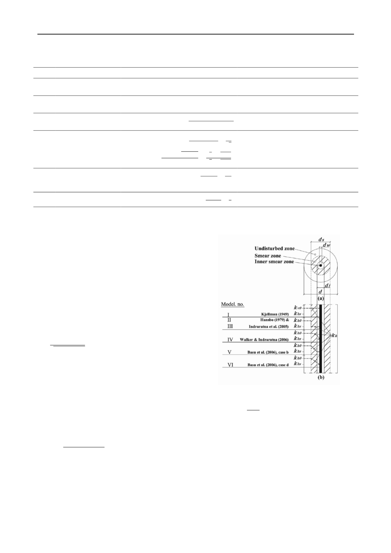
          Table 1. Characteristics and formulations of


            F


          in the investigated models (valid for
        
        
          10
        
        
          A
        
        
          and neglecting well resistance)
        
        
          no.


            Characteristics


            Formulation


          A


            Reference and comments


          I
        
        
          No smear zone,
        
        
          is
        
        
          used instead of
        
        
          B
        
        
          ( )
        
        
          Kjellman (1949), smear effects accounted for by
        
        
          adopting
        
        
          instead of
        
        
          II
        
        
          and constant
        
        
          in the smear zone
        
        
          (  ⁄ )         ( )
        
        
          Hansbo (1979), equal to model no. I for
        
        
          1
        
        
          III
        
        
          Equal to no. II,
        
        
          dependent on the void ratio
        
        
          (
        
        
          ⁄ )
        
        
          ⁄
        
        
          Indraratna et al. (2005), valid for normally con-
        
        
          solidated clays, equal to model no. II for
        
        
          ⁄
        
        
          IV
        
        
          Parabolic variation of
        
        
          in the smear zone
        
        
          (  ⁄ )       (   )
        
        
          (
        
        
          )  ( √ )
        
        
          (   )√ (   )
        
        
          (
        
        
          )  ( √  √
        
        
          √  √   )
        
        
          Walker and Indraratna (2006)
        
        
          V
        
        
          in the inner
        
        
          smear zone thereafter
        
        
          linear variation
        
        
          (  ⁄ )         ( )      ⁄    (   )
        
        
          Basu et al. (2006), case b, equal to model no. VI
        
        
          for
        
        
          1
        
        
          VI
        
        
          Linear variation
        
        
          (  ⁄ )           ⁄    (  )
        
        
          Basu et al. (2006), case d
        
        
          A
        
        
          ⁄


            ;


            &


            =initial stress & stress from the applied load;


            &


            =compression & permeability indices;


          ⁄
        
        
          B
        
        
          1.5 was used based on suggestions in Tavenas et al. (1983) for the anisotropy in permeability in homogeneous clays.
        
        
          Figure 1. a) Plan view of the unit cell; b) Vertical section of the unit cell
        
        
          and illustration of the analytical models investigated.