2012
Proceedings of the 18
th
International Conference on Soil Mechanics and Geotechnical Engineering, Paris 2013
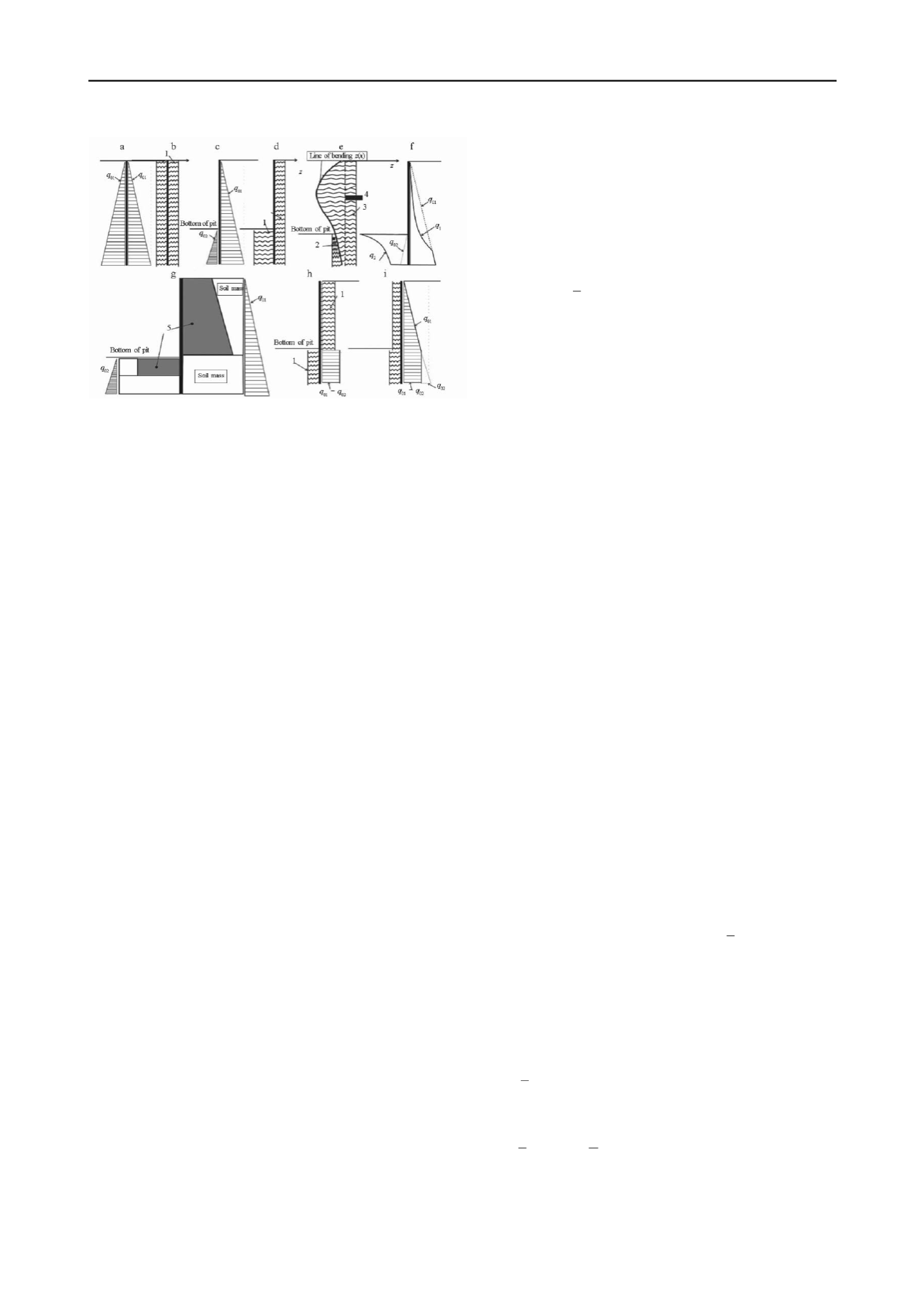
Figure 2. Steps in formulation of computational diagram: 1) elastic
prestressed springs; 2) and 3) compression and release of springs; 4)
position of enclosure prior to excavation of pit; 5) SCM.
Considering that the displacement of the soil and beam
below the bottom of the pit is less than that within the bounds of
the pit over its height, let us simplify the computational
diagram. The work of the springs on the outside of the pit below
its bottom can be neglected (Fig. 2, h), and replaced by a
constant pressure of the soil in a state of rest. If these springs are
eliminated from the computational diagram of the beam on the
outside of the pit, the pressure of the soil against the enclosure
below the bottom of pit will be q
0
= q
01
− q
02
, and the springs
on the inside beneath its bottom will be under no prestress.
To convert to the standard diagram of a beam on an elastic
bed, let us point out that the amount k*z by which the pressure
of the springs is reduced against the enclosure during release in
(2) is the reaction of ordinary springs with no prestress, which
are positioned on the opposite side when acted upon by force
q
01
. The work of the presstressed springs is than equivalent to
the work of stress-free springs under a load equal to the
prestress.
Consequently, the problem reduces to one of a beam on an
elastic bed (Fig. 2, i), where the beam represents the pit
enclosure, the external load is the lateral pressure of the
soil in a state of rest q
0
= q
01
− q
02
, and the coefficients of
the elastic bed are the stiffness coefficients k of the "SCM- soil"
system, which depend on the dimensions and shape of the SCM,
as well on the strength and deformation characteristics of the
soil. Considering the above, let is determine the following for
further analysis:
1) the active pressure against the "enclosure-SCM-soil"
system − the pressure q
0
of the soil at rest;
2) the contact pressure on the enclosure, which can be
transmitted through the SCM
q
=
q
0
−
kz
;
(3)
3) the reactive pressure of the SCM
−
that portion of
the active pressure against the system, which can be taken up
by the SCM as the system transitions to a new equilibrium
position after excavation of the pit
r
=
kz
.
(4)
Depending on the displacements of the enclosure, the soil
mass may function in an elastic stage, which can be described
by the work of elastic springs, or a plastic stage when the
contact pressure against the enclosure attains the active or
passive pressure of the soil. Since the basic purpose of SCM use
is to ensure preservation of surrounding development, the
stress-strain state (SSS) of the surrounding soil mass should not
go over into a plastic state, and the displacements of the
enclosure during excavation should be so small that
Coulomb's limiting equilibrium will not be realized. In the
analyses, therefore, only the elastic work of the system, where
the SCM ensures that the soil, and, accordingly, the "SCM-soil"
system, will function elastically, is ensured. This enables us to
perform the calculations in a linear statement, appreciably
simplifying solution of the problem of the optimal design of the
system under consideration.
In conformity with the physical essence of the problem, the
contact pressure against the enclosure above the bottom of the
pit cannot be less than zero (cannot act in the opposite direction
due to excavation of the pit). For stiffness coefficients above the
bottom of the pit should be satisfied the condition
q = q 0
−
kz > 0.
(5)
Using (5) the "enclosure-SCM-soil" system, therefore, it
is possible to use a finite-element formulation of a beam on an
elastic bed, where the lateral pressure of the soil in a state of rest
is the load.
Let us borrow terminology from (
Hogg and Arora 1983
) to
construct the mathematical optimal-design model. Terms of the
theory of matrix calculus can also be used when necessary.
In the computational model selected:
−
the
equation of state
is the matrix equation of the finite-
element method (FEM)
K(k)Z
−
Q = 0,
(6)
where
K
(
k
) is the global stiffness matrix of the system, the
elements of which will depend on
k
, and
Q
and
Z
are the vectors
of the nodal loads and displacements, respectively;
−
the
state variables
are the displacements
Z
at the nodes of
the finite-element diagram, which describe the behavior of the
system in question under load. The transposed form of the
vector
Z
= [
Z
1
, Z
2
, Z
3
, ..., Z m
] ,
(7)
where
m
is the number of degrees of freedom and state
variables
m
= 2
n
+ 2, and
n
is the number of finite elements.
After exclusion the angle of rotation from vector Z the vector z
of horizontal displacements expressed as follows
z
= [
Z
1
, Z
3
, ..., Z m
-1 ]= [
z
1
, z
2
, z
3
, ..., z n
+1 ];
(7a)
−
the
design variables
are contained in the set of
coefficients
k
, which describes the system itself, but not its
behavior.
k
= [
k
1
, k
2
, k
3
, ..., k n
] .
(8)
For the computational diagram under consideration, let us
write in the terms of the problem statement of an optimal finite-
dimensional design in state space.
It is required to determine the set of design variables k,
which will minimize the efficiency function, as determined
by the total stiffness coefficient with respect to all finite
elements of the model
ψ 0 = ψ 0 (k ) = ∑ k i → min, i =1...n
(9)
when state equations
h
(
k, z
) =
K
(
k)Z
−
Q
= 0
(10)
and constraints
ψ(
k, z
) = [ψ 1 (
Z
)
,
ψ 2 (
k
)
,
ψ 3 (
k
)
,
ψ 4 (
k, Z
)]
T
< 0
(11)
exist, where ψ(
k, Z
) is the set of itch type of constraints,
i
=
1-4.
Let us define the types of bounded functions.
1. Bounded-function vector ψ
1
(Z) is determined from the
conditions of the problem for which limits should be placed
on horizontal displacements
z
(7, a) at all
n
+ 1 nodes of the
enclosure, which is broken down into
n
elements. The
expressions ψ
1
(Z) are derived proceeding from the inequalities
z
1 <
S
max
, i
= 1
...n
+ 1
(12)
2. The vector function ψ
2
(
k
) reflects the limits placed on the
design variables
k
. Expressions for
ψ
2
(
k
) are derived, proceeding from the inequalities
k i
<
k
max
; k i > k
min
; i =
1
...e
,
(13)
where e is the number of the last element situated
above the base of the pit, kmax is the value defining
the upper limit of the variation of a variable, and k
min
= 0 is the
lower limit of variation in the absence of an SCM.


