2013
Technical Committee 207 /
Comité technique 207
3. The vector function ψ
3
(k) reflects the limits placed on the
design variables k below the bottom of the pit. The expressions
for ψ
3
(k) are derived from the inequalities
k
i
< k
max
; k
i
> k
min
; i = e + 1...n,
(14)
where k
min
is the lower limit of variation, and
k
min
= k
so
corresponds to the stiffness coefficient of
the soil when functioning elastically.
4. The vector function ψ
4
(k, Z) reflects the constraint that
ensures fulfillment of (5) − a reduction in pressure on the
elements residing above the base of the pit, and cannot exceed
the active horizontal load of the soil at rest on the corresponding
element. The expressions for ψ
4
(k, Z) are derived from the
inequalities
r
i
= k
i
*z
i
< q; i = 1...e + 1
(15)
where r
i
is the reduction in pressure, or the reaction
of the elastic bed at the itch node, k
i
is the coefficient of
the elastic bed at the itch node, and z
i
is the horizontal
displacement z (7, a) at the itch node.
In the problem under consideration, the limits are
represented by the following type of set:
ψ(
k, z
) = [ψ 1 (
Z
)
,
ψ 2 (
k
)
,
ψ 3 (
k
)
,
ψ 4 (
k, z
)]
(16)
Using (9), (10), and (16), the structure and analytical form of
the components of the mathematical optimal-design model are
entirely defined and ready for the solution.
2
PROBLEM SOLUTION
The search algorithm for optimization based on the method of
gradient projection, where that variation in design variables, for
which the efficiency function is decreased, and the limits are not
violated, is determined in each interval, is compiled for the
problem's solution, and is implemented in the software package
MATLAB v.7.9.0. The gradients of the efficiency and bounded
functions with respect to design variables are required for
construction of the algorithm are determined from analysis of
the sensitivity of the design in state space (
Hogg and Arora
1983
).
The search strategies consist in the plotting of a succession
of
k
p
points calculated in accordance with the rule
k p
+1 =
k p +
δ
k p , p
= 0, 1, ...,
(17)
where
p
is the number of iterations,
k
p
is a vector in the
form of (8), and δ
k
p
is the vector of variation in the design
variables, which decreases the efficiency function as determined
for each
p
using the gradients obtained from sensitivity analysis
of the design.
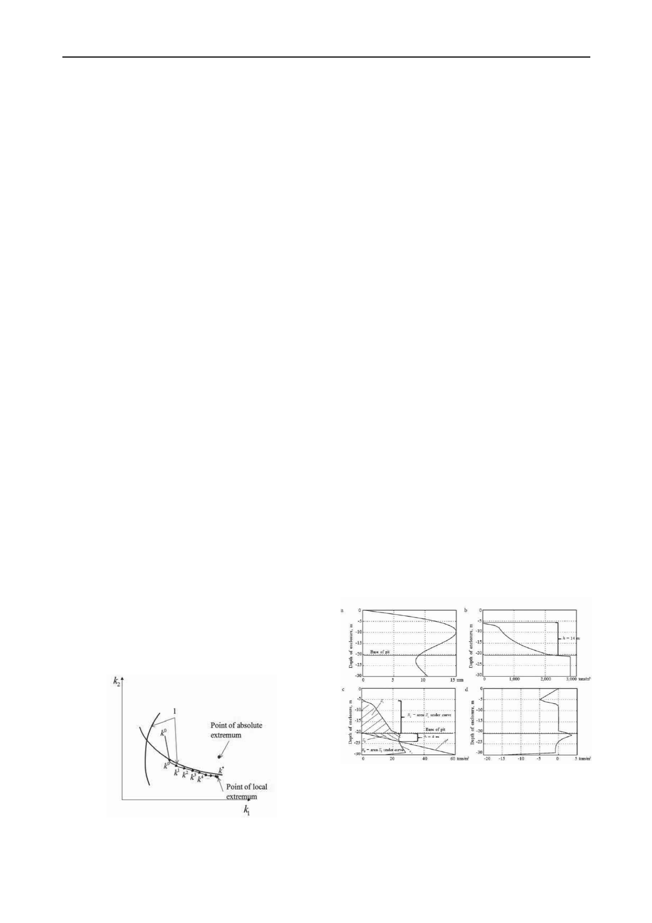
Figure 3 shows a geometric interpretation of the performance
of the algorithm for a two-dimensional space . The resultant
vector of the variation in the design δ
k
p
is obtained as a result
and the iteration process of the search for the conditional
extremum acquires the form shown in Fig. 3
Figure 3. Geometric interpretation of algorithm performance:
1) curve of bounded function;
After running the algorithm, the succession of points
converges on the optimal value of the efficiency function, i.e.,
the optimal distribution of
k
*
. As a result of running the
algorithm, the sequence of points converges to the optimal value
of the efficiency function, i.e., to the optimal distribution of the
coefficient
k
*
of the bed's stiffness.
The dimensions of the SCM corresponding to this stiffness
are required for determination of the optimal distribution of
the coefficient
k
. The following are basic initial data for
determination of the optimal dimensions of the SCM:
−
the minimum height
h
of the SCM, as determined above
and below the bottom of the pit based on the distribution curves
of
k
and the reactive pressure
R
;
−
the total reactive pressure of the SCM over the height
h
,
which should be taken up by the SCM as a component part of
the soil in order that the "SCM-soil" system correspond to the
elastic behavior
R =
∑
r i
,
(18)
where
i
is the number of nodes over the height
h
, and the
point of application of the force
R
resides at the level of the
center of gravity
r
of the plot; and,
−
the average displacement
z
avg
of the enclosure over height
h
, which corresponds to the displacement of the SCM under the
action of
R
z
avg
=
∑
z i
/
v
,
(19)
where
v
and
i
are the number of nodes, and the numbers of
the nodes over height
h
.
Use of
R
and
z
avg
enable us to convert to the assumption that
as a component part of the soil, the SCM functions as a solid
body, and is not calculated for individual elements over the
height.
It is therefore required to determine the minimum
dimensions of the SCM for which it will experience a horizontal
displacement
z
avg
under the horizontal force
R
.
Let us examine the application of the above-indicated
computational principles in an example of the calculation of
optimal SCM dimensions for the excavation of a pit in sand
with the following initial data: specific weight
γ
= 20 kN/m
3
,
overall compression modulus
E
= 25,000 kPa, angle of internal
friction in shear
ϕ
= 30°, cohesion
c
= 1.0 kPa, pit depth of 20
m, enclosure depth of 30 m, a "diaphragm wall" enclosure with
a thickness of 800 mm, and an upper thrust bracing consisting
of a reinforced concrete span with a thickness of 500 mm.
Solution of the optimal-design problem (Fig. 4) includes
curves of enclosure displacements (Fig. 4, a), distributions of
the optimal stiffness coefficient over the height of the enclosure
(Fig. 4, b), the reactive pressure (Fig. 4, c), and the contact
pressure (Fig. 4, d).
Figure 4.
Results of calculation for
S
max = 15 mm
: а) displacement; b)
stiffness coefficient diagram; c) reactive pressure; d) contact pressure
To determine the optimal dimensions, let us examine the
SCM above and below the bottom of the pit.
According to the plot (Fig. 4, b), the SCM above the bottom of
the pit extends to the point along the height where
k
= 0 and
h
=
14 m. For the enclosure above the bottom of the pit where
k
= 0,
no soil cement is required. Let us consider the SCM a massive
retaining wall 14 m high, the upper and lower bases
a
and
b
of
which should be determined from calculation of (18) for a


