2844
Proceedings of the 18
th
International Conference on Soil Mechanics and Geotechnical Engineering, Paris 2013
2 DEVELOPMENT OF A MULTI-METHOD
AUTOMATED TOOL FOR TRAVEL TIME ANALYSES
A new software tool was developed by GDS Instruments to
perform automated analyses of bender element test data. The
primary aim of this tool was to allow travel time estimations to
be conducted objectively via a simple user interface, providing
both visual and numerical representations of the estimated travel
times. Implementation of the tool was completed by creating
Add-Ins for Microsoft Excel, a decision based on the ubiquitous
use of the software.
Based on the recommendations presented in Section 1.1, it
was considered important to include a number of analysis
methods within the tool, providing flexibility to the user when
interpreting the results. Variations of the three primary
approaches listed in Section 1.1 were therefore chosen for
implementation: observation of points of interest within the
received wave signal via software algorithm (TD); cross-
correlation of the source and received signals (TD); group travel
time calculation obtained from the absolute cross-power
spectrum phase diagram (FD). Implementation of these methods
is briefly discussed in Section 2.2 and 2.3, whilst the analysis
tool is introduced in Section 2.1.
2.1
GDS Bender Element Analysis Tool user interface
The GDS Bender Element Analysis Tool (BEAT) is accessed
via two Add-Ins for Microsoft Excel (version 2007 or later): the
Interactive Analysis tool and the Batch Analysis tool. The
Interactive Analysis tool is designed to analyse one BE test at a
time, whilst allowing the user some interaction when
performing the FD estimation. To use the tool, BE test data is
firstly imported into Excel, with relevant test parameters then
selected via the window interface displayed in Figure 1. Note
this allows data obtained from any BE system to be analysed,
assuming the data file can be loaded within Excel. The tool then
performs the majority of the analysis before pausing to allow
user alteration of the frequency window chosen for the FD
estimation.
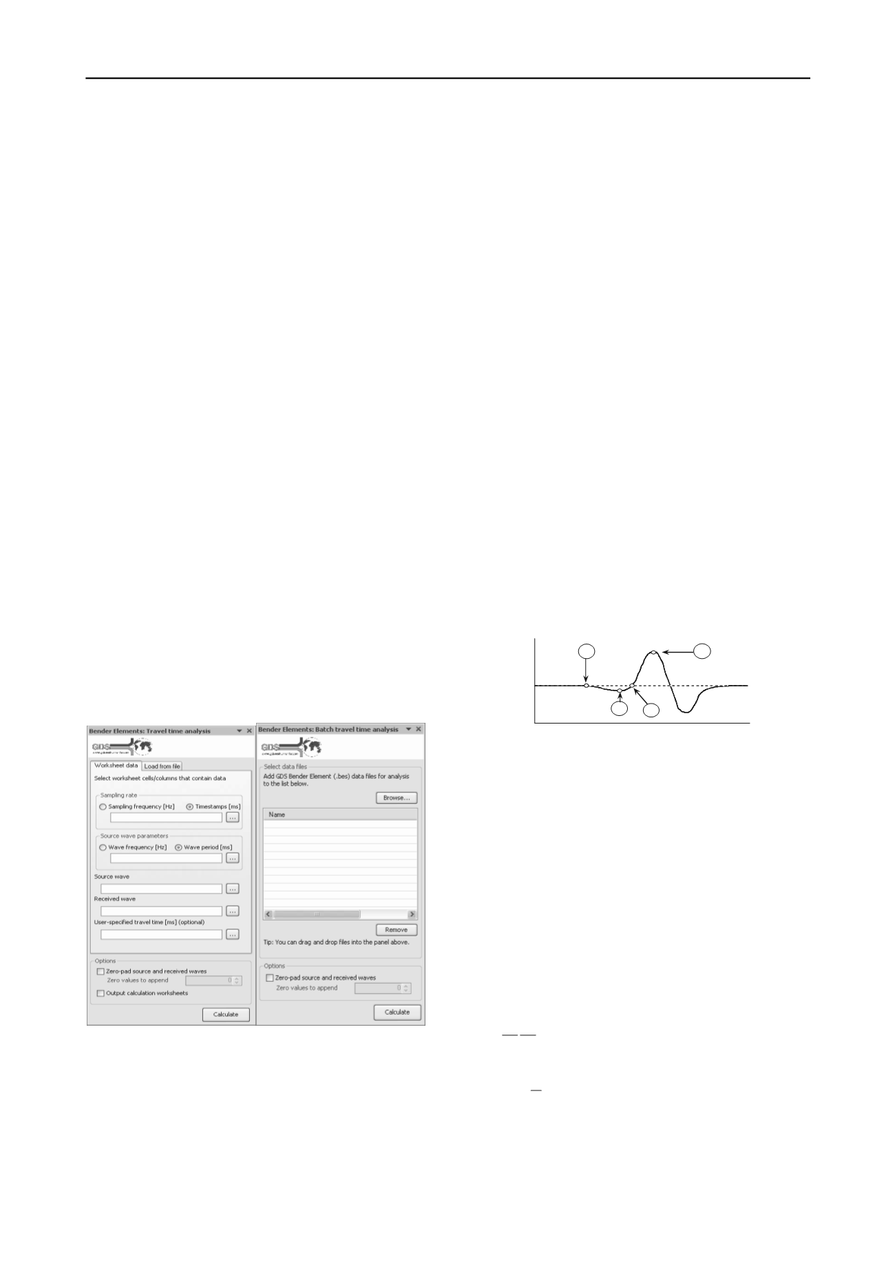
Figure 1. Interactive Analysis (left) and Batch Analysis (right)
parameter / data file input windows within Microsoft Excel.
Conversely the Batch Analysis tool is designed to analyse
multiple BE tests at a time, assuming the data is organised using
the GDS Bender Element System (BES) output format (.bes).
The tool is used by simple loading .bes files into the window
interface shown in Figure 1 and clicking “Calculate”.
2.2
Observation of received wave signal via algorithm
Figure 2 displays an idealised received shear wave signal
containing the near field effect, with four points of interest
noted: first deflection (A); first bump maximum (B); zero after
first bump (C); major first peak (D) (Lee and Santamarina
2005). To observe the time at which each point occurs, relative
to initial triggering of the source signal (time zero), an
algorithm was included within BEAT to implement the
following procedure:
- The major first peak (D) is located by scanning the
signal and determining the maximum (i.e. most
positive) output. The time signature corresponding to
this maximum thus defines point D.
- Point B is determined next by scanning the signal from
time zero up to point D and locating the minimum (i.e.
most negative) output. The corresponding time
signature defines point B.
- Point C is then found by scanning the signal between
point B and point D to locate the output closest to zero.
The corresponding time signature defines point C.
- Point A is located via an iterative process: beginning at
time zero, the mean and standard deviation of 10
consecutive outputs (e.g.
n
1
–
n
10
) are calculated, with
the subsequent five outputs (
n
11
–
n
15
) then assessed to
determine whether all are at least three standard
deviations more negative than the calculated mean. If
‘true’, the time signature of the first of the five
subsequent outputs (i.e.
n
11
) is used to define point A; if
‘false’, the iteration proceeds by determining the mean
and standard deviation of the next set of 10 consecutive
outputs (i.e.
n
2
–
n
11
) until a ‘true’ condition is reached.
C B
D
Output
Time
A
Figure 2. Idealised received shear wave signal containing the near field
effect (reproduced from Lee and Santamarina 2005).
2.3
Cross-power spectrum and cross-correlation of source
and received wave signals
Use of the cross-power spectrum and cross-correlation functions
to provide travel time estimations has been extensively covered
in the literature (Viggiani and Atkinson 1995, Leong et al.
2005), and as such only the two primary equations relating to
each method used within BEAT are presented here. Equation 2
firstly displays the group travel time,
t
g
, where
dφ/df
corresponds to the slope of the absolute cross-power spectrum
phase diagram across a user-defined frequency range. Equation
3 provides the discrete cross-correlation function,
CC
xy
, with
respect to source signal time shift,
t
s
, where
T
corresponds to the
signal time record and
Y(T)
and
X(T)
correspond to the source
and received signal outputs respectively.
df
d
t
g
2
1
(2)
)
()(
1 )(
1
0
T
T
s
s xy
tTYTX
T
t CC
(3)
The time shift corresponding to the maximum value of
CC
xy
is used for the travel time estimate obtained from the TD
analysis (i.e.
t
=
t
s
when
CC
xy
= maximum), whilst a frequency
window running from 0.8 to 1.2 times the source signal
frequency is used to determine the group travel time
t
g
=
t


