2845
Technical Committee 212 /
Comité technique 212
(unless the user alters this frequency window when using the
Interactive Analysis tool).
2.4
GDS Bender Element Analysis Tool output
Following the analysis process, BEAT produces two output tabs
within Excel: these are Travel Time Report and Graphs. The
Travel Time Report lists all relevant data numerically, including
the data filenames, travel time estimates obtained from the TD
and FD analysis methods, and various analysis metrics. The
Graphs tab displays a number of plots for each data file,
including the source and received wave signals with travel time
estimates shown, frequency spectrums for each signal, the
unwrapped phase angle, and values of the cross-correlation
function. These outputs allow the user to further assess the
validity of the analysis, and to use the travel time estimates in
V
S
and
G
0
calculations.
3 BENDER ELEMENT TESTS ON LEIGHTON BUZZARD
SAND TRIAXIAL SPECIMEN
To initially assess the performance of BEAT, a series of bender
element tests were performed on a triaxial specimen of Leighton
Buzzard sand Fraction D. The triaxial apparatus used was a
GDS Dynamic Triaxial Testing System (DYNTTS), with
bender element tests conducted via a GDS BES. The specimen,
nominally 70 mm diameter by 144 mm in height, was prepared
using a moist-tamping method similar to that previously
employed by the authors (Rees 2010). Following saturation (B
value
≥
0.95), the specimen was isotropically consolidated to
four mean effective stresses,
p’
, with bender element tests being
conducted at each stress level. The data presented herein
focuses exclusively on the tests performed at
p’
= 100 kPa using
a single sine-wave source.
Properties of the specimen are presented in Table 1,
including void ratio,
e
, and relative density,
D
r
. Note values of
the maximum and minimum void ratios used to estimate
D
r
were 1.01 and 0.72 respectively (Klotz 2000), with
L
equal to
the element tip-to-tip distance.
Table 1. Properties of the Leighton Buzzard sand triaxial test specimen.
p’
(kPa)
e
D
r
(%)
ρ
(t/m
3
)
L
(mm)
100
0.88
± 0.03
43
± 10
1.88
± 0.02
139.1
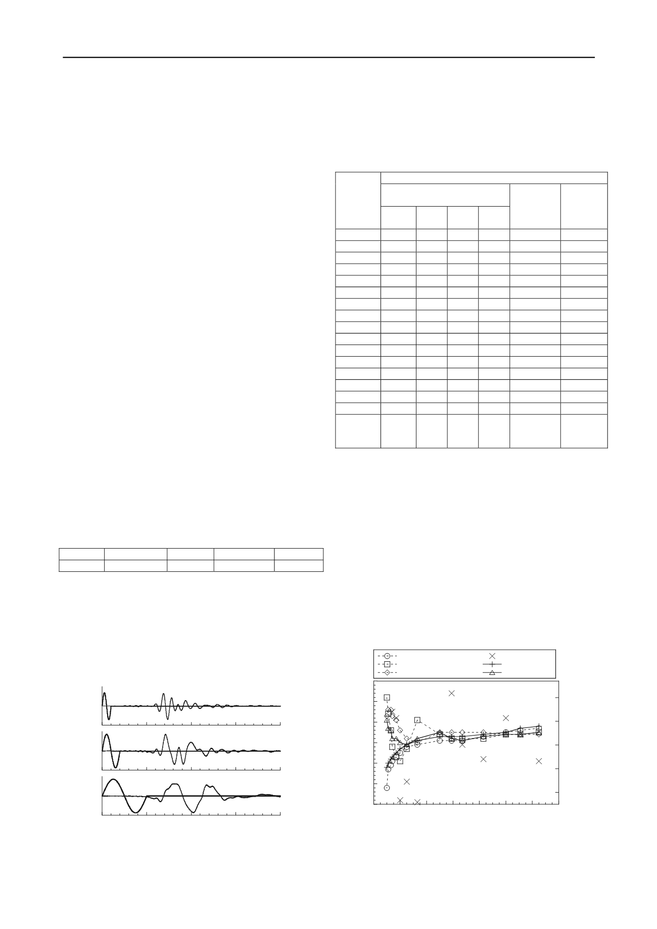
The bender element tests were conducted by systematically
varying the source wave frequency, as recommended by TC-29,
from the chosen values of 14.3 kHz to 1.0 kHz. For each test
frequency five separate source element triggers were applied to
the specimen, with the received signal output then stacked in the
time domain to remove random signal noise. Three examples of
source and received signals obtained during these tests are
presented in Figure 3.
Sine:
f
= 10.0kHz
Sine:
f
= 5.0kHz
Sine:
f
= 2.0kHz
500
1000
1500
Time (
s)
Figure 3. Source and received bender element signals obtained from the
test specimen at
p’
= 100 kPa.
After completion of the bender element tests, the Batch
Analysis Add-In tool was used to automate the data analysis and
report the estimated travel times. Note the analysis was
completed after approximately 45 seconds using a desktop PC
running Windows XP SP3 with a 2.93 GHz Intel Core 2 Duo
CPU and 2.00 GB RAM. Travel time estimates obtained from
this process are presented in Table 2.
Table 2. Travel time estimates from the Batch Analysis tool.
Shear wave travel time estimates,
t
(µs)
Observation of Received Signal
(TD)
Source
f
(kHz)
Point
A
Point
B
Point
C
Point
D
Cross-
correlation
(TD)
Cross-
spectrum
(FD)
14.3
221
635
651
675
662
620
12.5
224
637
655
681
663
703
11.1
224
641
658
685
663
663
10.0
225
643
662
689
662
641
8.3
227
646
667
698
662
697
6.7
226
652
671
706
661
678
5.9
278
650
671
712
662
613
5.0
497
650
672
713
662
495
3.3
227
653
676
719
674
771
2.5
229
654
682
784
669
735
2.0
488
655
690
828
657
767
1.7
450
657
696
846
645
642
1.4
404
658
700
855
640
633
1.3
398
659
707
858
632
515
1.1
442
658
716
862
632
325
1.0
443
659
744
868
640
235
Scatter
for
f
≥
3.3kHz :
± 138
± 9
± 13
± 22
± 7
± 138
To compare the performance of BEAT with subjective
analyses, a geotechnical academic at Warsaw University (WU)
with previous bender element signal analysis experience was
sent the test data (from 12.5 kHz – 1.0 kHz) and asked to
provide travel time estimates using any observational, non-
automated analysis methods they considered appropriate. This
resulted in travel times being estimated with five separate
methods, including the first arrival or start-to-start method
(specified as point C in Figure 2) and the peak-to-peak
technique. Travel time estimates produced by BEAT and the
subjective analyses from WU were subsequently used to
calculate
V
S
and
G
0
values, which are presented in Figure 4. It
should be noted a system delay of 42 μs was subtracted from all
travel time estimates when calculating
V
S
, and that
G
0
values are
approximate (± 2 MPa) due to axis scaling when plotting both
parameters in Figure 4.
190
200
210
220
230
240
250
70
90
110
0
2
4
6
8 10 12 14
Point C (BEAT)
Peak-to-peak (BEAT)
Cross-correlation (BEAT)
Phase-angle (BEAT)
Point C (WU)
Peak-to-peak (WU)
Shear wave velocity,
V
S
(m/s)
Approximate small-strain
shear modulus,
G
0
(MPa)
Source frequency,
f
(kHz)
Figure 4. Shear wave velocity and approximate small-strain shear
modulus values calculated from estimated travel times.


