 
          2770
        
        
          Proceedings of the 18
        
        
          th
        
        
          International Conference on Soil Mechanics and Geotechnical Engineering, Paris 2013
        
        
          moment function,


          , is a first order polynomial, Eq. (13) is
        
        
          solved by second integral with a single Gaussian point as


           = 


          =


          ′


          (13)
        
        
          where


          =


          or


          in Eq. (13),
        
        
          ′
        
        
          is the weight for the single
        
        
          Gaussian point (i.e.,
        
        
          ′
        
        
          = 2.0, referring to Table 1), and


          is the
        
        
          sensor position projected from the Gaussian point in the range
        
        
          between 0 to


          . Note that


          is in the middle of the target length
        
        
          according to Table 1. Figure 6 shows the exact locations of


          in
        
        
          the testing configuration.
        
        
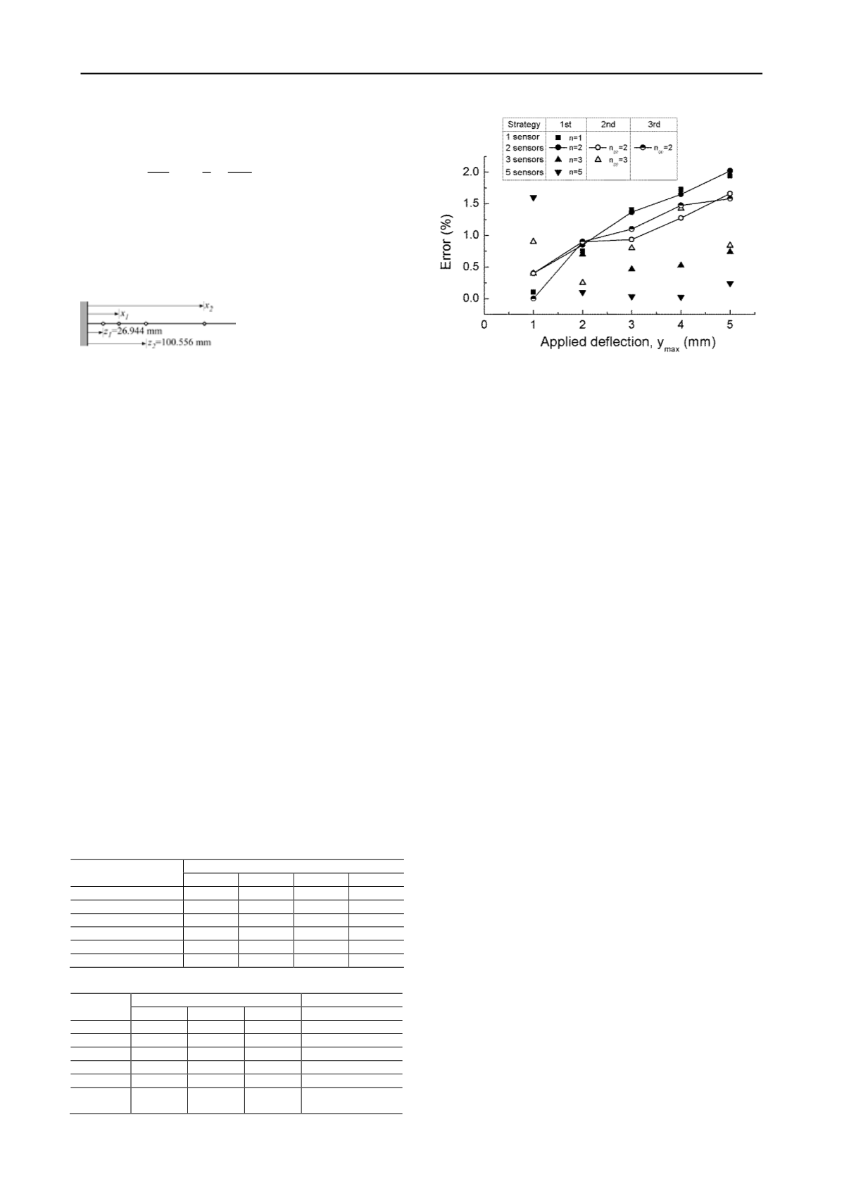
          Figure 6. Optimal location of the sensors for cantilever beam
        
        
          According to the different configurations for three different
        
        
          strategies illustrated in Figures 5 and 6, the FBG sensors were
        
        
          inscribed on the optic fiber attached to the bar specimen, and
        
        
          then the displacement was applied repeatedly by more than ten
        
        
          times. Table 4 compares applied and calculated values of


          for the configurations with sensors positioned at the regular
        
        
          intervals. As the number of sensor increases, the error
        
        
          significantly decreases. Figure 7 shows the variation of errors
        
        
          against increasing applied deflection. When employing one or
        
        
          two sensors, the error increases as the applied deflection
        
        
          increases. When three or five sensors are used, the errors remain
        
        
          approximately constant irrespective of applied displacement.
        
        
          Table 5 compares the applied and calculated values of


          for the configurations with sensors positioned at the projected
        
        
          Gaussian points. Even in this case, the errors are also decreasing
        
        
          as the number of the sensors increases. For the same number of
        
        
          sensors, however, the error in the configuration according to the
        
        
          second strategy is smaller than that for the first strategy. This
        
        
          implies that positioning sensors deployed via the analytical
        
        
          formula exhibits better performance than uniformly distributed
        
        
          sensors.
        
        
          As shown in Table 5, the error of sensors deployed with the
        
        
          third strategy yields much better performance than others. The
        
        
          average error for the third strategy is smaller by 0.2% than the
        
        
          error for the first strategy, and even smaller than the error for
        
        
          the second strategy by 0.03%. It is obvious that measuring
        
        
          displacement rigorously based on the Gaussian quadrature rule
        
        
          is superior to other cases because of its simple calculation,
        
        
          whereas the results indicates that increasing the number of
        
        
          sensors uniformly would give better measurement than
        
        
          employing the Gaussian quadrature rule.
        
        
          Table 4. y
        
        
          max
        
        
          , using sensors positioned at the regular intervals
        
        
          Applied
        
        
          y
        
        
          max
        
        
          , mm
        
        
          y
        
        
          max
        
        
          using 1
        
        
          st
        
        
          strategy
        
        
          n=1
        
        
          n=2
        
        
          n=3
        
        
          n=5
        
        
          1
        
        
          0.999
        
        
          0.996
        
        
          0.996
        
        
          1.016
        
        
          2
        
        
          1.985
        
        
          1.983
        
        
          1.986
        
        
          2.002
        
        
          3
        
        
          2.958
        
        
          2.959
        
        
          2.986
        
        
          2.999
        
        
          4
        
        
          3.931
        
        
          3.934
        
        
          3.979
        
        
          3.999
        
        
          5
        
        
          4.903
        
        
          4.899
        
        
          4.963
        
        
          4.988
        
        
          Average error, % 1.18
        
        
          1.25
        
        
          0.54
        
        
          0.28
        
        
          Table 5. y
        
        
          max
        
        
          , using sensors positioned at projected Gaussian points
        
        
          Applied
        
        
          y
        
        
          max
        
        
          , mm
        
        
          y
        
        
          max
        
        
          using 2
        
        
          nd
        
        
          strategy
        
        
          Using 3rd strategy
        
        
          n
        
        
          gp
        
        
          =1
        
        
          n
        
        
          gp
        
        
          =2
        
        
          n
        
        
          gp
        
        
          =3
        
        
          n
        
        
          gp
        
        
          =2
        
        
          1
        
        
          0.999
        
        
          0.996
        
        
          0.991
        
        
          1.000
        
        
          2
        
        
          1.985
        
        
          1.982
        
        
          1.995
        
        
          1.982
        
        
          3
        
        
          2.958
        
        
          2.972
        
        
          2.976
        
        
          2.967
        
        
          4
        
        
          3.931
        
        
          6.949
        
        
          3.943
        
        
          3.941
        
        
          5
        
        
          4.903
        
        
          4.917
        
        
          4.958
        
        
          4.921
        
        
          Average
        
        
          error, %
        
        
          1.18
        
        
          1.04
        
        
          0.84
        
        
          1.01
        
        
          Figure 7. Errors in measurement using three different strategies
        
        
          3 CONCLUSION
        
        
          Using multiplexed FBG sensors require a careful deployment
        
        
          scheme to minimize errors in measuring lateral displacement of
        
        
          the pile through the least number of sensors. Herein, a new
        
        
          approach to deploy the FBG sensors for measurement of lateral
        
        
          displacement of piles was introduced. The Gaussian quadrature
        
        
          formula was adopted to minimize the error in measuring the
        
        
          deflection of a laterally loaded pile. The performance of
        
        
          Gaussian quadrature formula for optimizing sensor positions
        
        
          has been tested using the aluminum bar specimen representing a
        
        
          lab-scale cantilever beam with the clamped end. Primary
        
        
          objective for sensor deployment was set to minimize the error in
        
        
          measuring the maximum deflection at the point of loading.
        
        
          Three optimization strategies—positioning sensors at regular
        
        
          intervals, positioning sensors at projected Gaussian points but
        
        
          not following the Gaussian rule, and positioning sensors exactly
        
        
          based on the Gaussian rule—were implemented. In both cases
        
        
          for the first and second strategies, the measurement error
        
        
          decreases as the number of sensors increases. For the same
        
        
          number of sensors, however, the second strategy where the
        
        
          sensors were positioned at the projected Gaussian points
        
        
          reduces the errors by 0.2% than those for the first strategy.
        
        
          Positioning the sensors rigorously based on the Gaussian
        
        
          quadrature rule enhances the accuracy more than just using the
        
        
          Gaussian points. The experimental results suggested that the
        
        
          analytical deployment plan using the Gaussian quadrature rule
        
        
          can be helpful in crafting a placement in measuring the
        
        
          displacement of the laterally loaded pile accurately.
        
        
          4 ACKNOWLEDGEMENTS
        
        
          This work was supported by the National Research Foundation
        
        
          of Korea (NRF) grant funded by the Korean government
        
        
          (MEST) (No. 2009-0090774)
        
        
          5 REFERENCE
        
        
          Abramowitz, M. and Stegun, I.A. (1972), Handbook of Mathematical
        
        
          Functions, Dover, ISBN 978-0-486-61272-0
        
        
          Chung, W., Kang, D.H., Choi, E.S., Kim, H.M. (2005), “Monitoring of
        
        
          a steel plate girder railroad bridge with fiber bragg grating sensors,”
        
        
          Journal of Korean Society of Steel Construction, Vol. 17, No. 6, pp.
        
        
          681-688.
        
        
          Habel, W.R. and Krebber, K. (2011), “Fiber-optic sensor applications in
        
        
          civil and geotechnical engineering,” Photonic sensors, Vol. 1, No. 3,
        
        
          pp. 268-280.
        
        
          Lee, W., Lee, W.-J., Lee, S.-B., and Salgado (2004), “Measurement of
        
        
          pile load transfer using the Fiber Bragg Grating sensor system,”
        
        
          Canadian Geotechnical Journal, Vol. 41, No. 6, pp. 1222-1232.