 
          2769
        
        
          Technical Committee 212 /


            Comité technique 212


          Figure 1. A cantilever beam with a concentrated load, simulating the
        
        
          pile subjected to a lateral load.
        
        
          2 EXPERIMENTAL SETUP
        
        
          2.1


            Experimental procedure


          A model cantilever beam is the aluminum bar specimen which
        
        
          has a physical properties listed in Table 1. Figure 1 shows the
        
        
          loading system including a clamp to fix one end of the bar and a
        
        
          calipers used to apply the displacement on the other end of the
        
        
          bar. In the middle points, two dial indicators were attached to
        
        
          measure the deflections of the bar during loading. Because the
        
        
          displacement is applied by using the calipers, the concentrated
        
        
          load, P, can be estimated as


            P


          = 3


          /


          . An optic fiber
        
        
          including FBG sensors inscribed at given positions was epoxied
        
        
          on the top surface of the bar specimen developing tensile strains
        
        
          during loading. Electric strain gages were glued together to
        
        
          validate the performance of the FBG sensors.
        
        
          Figure 3. A model cantilever beam system.
        
        
          Table 2. Properties of aluminum bar speciment
        
        
          Length,


            l


          (mm)
        
        
          255
        
        
          Thickness,


            h


          (mm)
        
        
          6
        
        
          Width (mm)
        
        
          25
        
        
          Young’s Modulus,


            E


          (Gpa)
        
        
          70.56
        
        
          Moment of inertial,


            I


          (mm
        
        
          4
        
        
          )
        
        
          450
        
        
          Bending stiffness,


            EI


          (N
        
        
          ·
        
        
          mm
        
        
          2
        
        
          )
        
        
          31,752,000
        
        
          As in Eq. (11), the lateral displacement, y, is obtained by
        
        
          integrating Eq. (10) which is a polynomial equation with degree
        
        
          2 so that two Gaussian points,
        
        
          ξ
        
        
          1
        
        
          = -0.577 and
        
        
          ξ
        
        
          2
        
        
          = +0.577, are
        
        
          possibly chosen according to Table 1. As shown in Figure 4,
        
        
          sensors were located at two points projected from two Gaussian
        
        
          points. The FBG sensors measure the strains via Eq. (3). When
        
        
          the point load, P, is applied, the cantilever beam specimen is
        
        
          deflected. The curvature, 1/
        
        
          ρ
        
        
          , at a section can be calculated by
        
        
          the strains developed on upper and lower surfaces as


          =


          =


          (12)
        
        
          where


          is the tensile strain on upper surface,


          is the
        
        
          compressive strain on lower surface of the bar, and


            h


          is the
        
        
          thickness of the section of the bar specimen. Assuming that both
        
        
          tensile and compressive strains have the same magnitude, the
        
        
          sensors were attached only on the upper surface of the bar
        
        
          specimen. Consequently, the moment at the sections where the
        
        
          sensors were placed can be measured as
        
        
           = 2


          /ℎ
        
        
          .
        
        
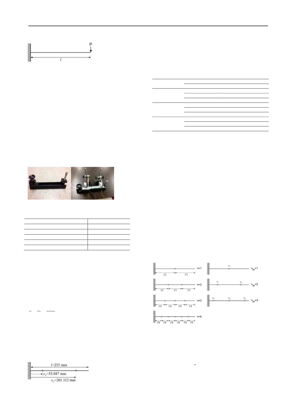
          Figure 4. Optimal sensor positions for a cantilever beam
        
        
          For a given displacement, theoretical values of the moment can
        
        
          also be computed via Eq. (9) and (11), thus
        
        
           = 3


           −
        
        
          /


          for a given


            y


            max


          value. As shown in Table 3, errors in the
        
        
          measured moment to computed moment range between 0.15
        
        
          and 1.54%, and average out to 0.82%.
        
        
          Table 3. Measured and computed moments at two Gaussian points
        
        
          Applied
        
        
          deflection,


            y


            max


          Moment, N-mm
        
        
          Sensor position


            x


            1


            x


            2


          1 mm
        
        
          Measured
        
        
          1153.6
        
        
          295.3
        
        
          Computed
        
        
          1155.3
        
        
          309.6
        
        
          Error, %
        
        
          0.15
        
        
          0.46
        
        
          2 mm
        
        
          Measured
        
        
          2290.4
        
        
          612.8
        
        
          Computed
        
        
          2310.7
        
        
          619.2
        
        
          Error, %
        
        
          0.88
        
        
          1.03
        
        
          3 mm
        
        
          Measured
        
        
          3435.6
        
        
          914.458
        
        
          Computed
        
        
          3465.9
        
        
          928.8
        
        
          Error, %
        
        
          0.88
        
        
          1.54
        
        
          2.2


            Optimizing sensor positions using Gaussian points


          Primary objective for deployment in this study is to minimize
        
        
          the error in measuring the maximum deflection at the point of
        
        
          loading,


          . Herein, we developed three optimization
        
        
          strategies. The first strategy is positioning sensors at regular
        
        
          intervals, which is a simplest way to deploy. The second is
        
        
          positioning sensors at projected Gaussian points but not
        
        
          following the Gaussian quadrature rule. The third is positioning
        
        
          sensors exactly based on the Gaussian quadrature rule.
        
        
          Figure 5 illustrates different deployment schemes according
        
        
          to first and second strategies. Four possible schemes at regular
        
        
          intervals are illustrated in figures on the left-hand-side column
        
        
          of Fig. 5, where n is the number of sensors used for each
        
        
          scheme. Figures on the right-hand-side column of Fig. 5
        
        
          illustrate three deployment schemes using the projected
        
        
          Gaussian points for the number of Gaussian points,


            n


            gp


          = 1, 2,
        
        
          and 3. For each case, the FBG sensors on a single strand were
        
        
          inscribed at positions marked as open symbols in Fig. 5. After
        
        
          applying


          by the calipers, the strain at each sensor position
        
        
          was measured by FBG sensors. Subsequently two unknowns
        
        
          such as


            P


          and


            l


          in Eq. (8) were determined by using measured
        
        
          strains incorporated with the boundary condition at the clamped
        
        
          end, and then


          was calculated via Eq. (11).
        
        
          Figure 5. Different sensor deployments at regular and Gaussian points
        
        
          The third strategy requires a double integral to calculate


          using the moment values as described in section 2.3. Using the
        
        
          Gaussian quadrature rule,


          can be obtained by integrating
        
        
          the slope function, S, which is the polynomials of degree 2, as


          =  


          =


          [


           + 


          ]
        
        
          (13)
        
        
          where


          and


          are weights for two Gaussian points given in
        
        
          Table 1, and


          and


          are the distances from the clamped end
        
        
          to projected Gaussian points as illustrated in Fig. 4. Because the