847
Technical Committee 103 /
Comité technique 103
4
s
v
4
0
0 f
κ λ κ M d
d =
+
1+ 1+ M
p
ε
e
e
p
(7)
states of clays are initially on INCL, the reloading line w
4.2 Delayed strain
represent the data of an oedometer
(
here
e
λ
is the void ratio of the point on INCL at current
p
,
t
the
n
to
ov
(9)
here
denotes the aging time and
If
ill
coincide with INCL.
Dots in Figure 5
consolidation test on clays (Zhu 2000). The process before C
belongs to the primary compression AC in Figure 2, and the one
after C is the secondary compression CD. In the semi-
logarithmic coordinate system, the data points of CD form a line
approximately. So the formula of the creep can be expressed as
e
C ln( 1)
e e
t
8)
w
time and C
αe
the coefficient of secondary compression.
Clays
develop
from
normal
consolidatio
erconsolidation with creeping. The time effects on clays are
equivalent to making clays stiff and aged. So the elapsed time
of the creep is called the aging time. It was pointed out that the
creep rate is dependent on the current state and independent of
the paths (Yin et al. 2002). Therefore, the state of clays can be
represented by one path, e.g. the path of creep. That is, the state
of clays is able to be described by the aging time. Besides, in
e
-
ln
p
plane,
R
can also reflect the state of clays. Hence, the aging
time and
R
are related with each other. The relationship between
them can be derived as
-α
a
1
t
R
w
a
t
e
C
.
erived from e (8) and
(9)
The elayed strain increment is d
qs.
d
, as shown as follows:
tp
α
e
a
e
v
0 a
0
C d
C
d =
d
1+ +1 1+
t
ε
R t
e t
e
(10)
e
0
e
1
e
2
e
3
e
4
e
5
e
6
e
7
e
8
e
9
e
10
e
11
1.05
1.10
1.15
1.20
1.25
1.30
1.35
1.40
Figure 5. Experimental data of isotropic consolidation tests Zhu 2000).
(
10
100
1000
0.7
0.8
0.9
1.0
1.1
1.2
Rate: %/h
Infinity
5.70
1.14
10 -1
5.70
10 -3
where d
t
a
is the aging time increment, and d
t
the real time
increment. Although the aging time is not equal to the real time,
the increments of them are the same.
4.3 1-D stress-strain-time relationship
By combining eqs. (6), (7) and (10), the 1-D stress-strain-time
relationship of OC clays can be expressed as
4
α e
v
4
0
0
0
f
C
κ d λ κ M d
d =
+
+
d
1+
1+
1+
M
p
p
ε
R t
e p
e
p
e
(11)
If clays are loaded instantaneously, i.e., d
t
=0, then the
relationship will be changed into the stress-strain relationship of
the UH model.
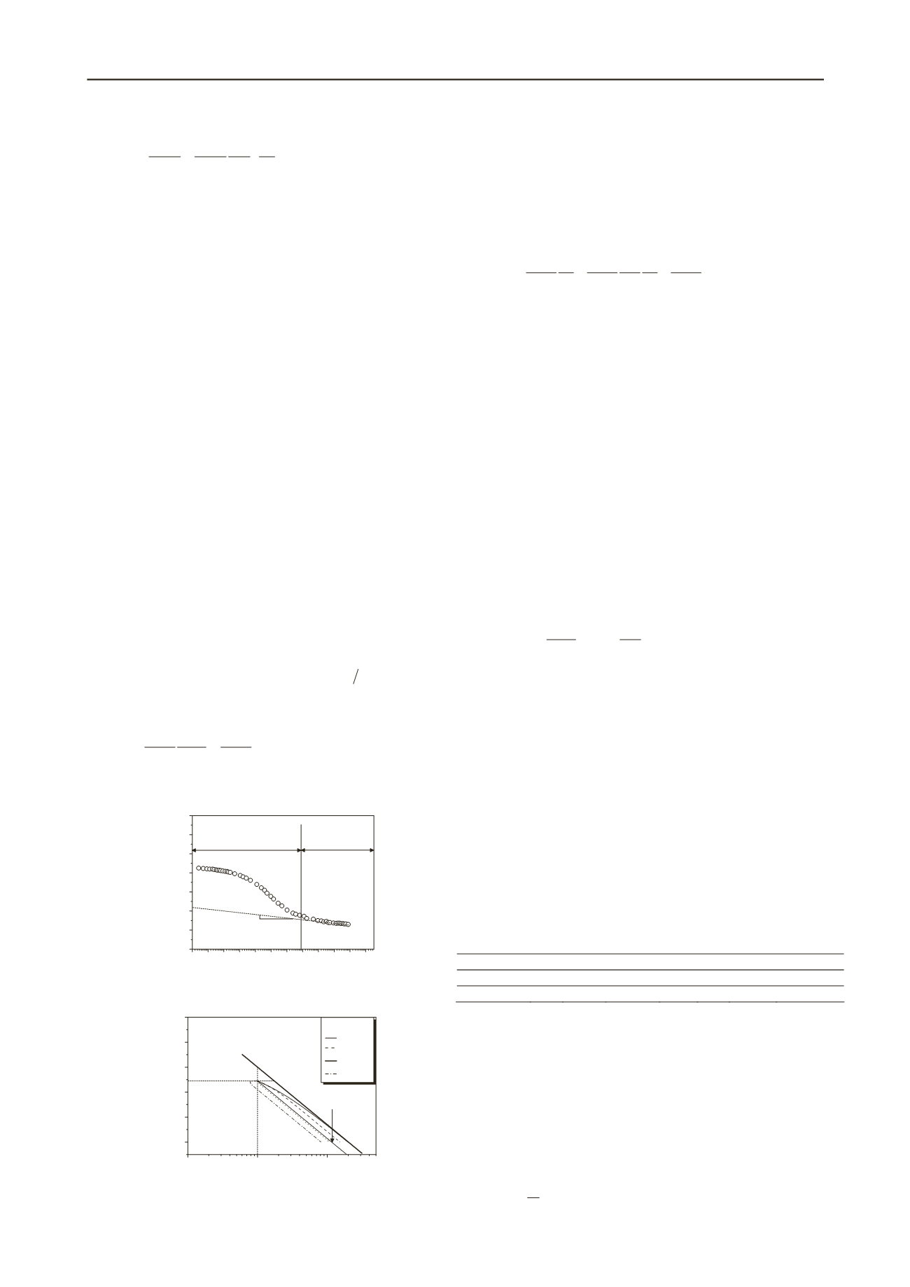
4.4 1-D prediction
Figure 6 shows the predicted results of isotropic compressions
on OC clays (initial
R
=0.5) at constant rates of void ratio. The
row “1-D” in Table 1 illustrates the values of parameters used in
the prediction.
4.4.1 Characteristic rate
In Figure 6 the compression curves of different rates are parallel
to INCL finally. When the rate is larger, as curve “5.70 %/h”
shows, clays show overconsolidated behaviors. When the rate is
slower, as curve “1.14×10
-1
%/h” shows, clays behave in a
similar way of underconsolidated clays. If clays just behave as
normal consolidation when being compressed with a certain
rate, then the certain rate will be defined as the characteristic
rate. The characteristic rate is a function of
R.
-1 4
α
cr
e
4
f
λ
M
= C
1
λ κ
M
e
R
(12)
When the states of clays are on INCL, M
f
=M so that the
characteristic rate is infinite, which means the instant
compression curve goes back to INCL at last.
4.4.2 Relaxation
If clays are being isotropically compressed at a very slow rate,
as curve “5.70×10
-3
%/h” in Figure 6, on the curve there will be
a part where
e
is almost invariant but
p
is decreasing. At this
time, the behavior of clays is similar to relaxation. The
difference between this type of curves and other curves is that
the beginnings of the former lie on the left of the creep path,
which indicates that the creep path is a boundary determining
whether the relaxation exists. Consequently, during the isotropic
compression, if the current strain rate of clays is smaller than
the creep rate, then the loading curve will exhibit the relaxation
feature.
Table 1. Parameters adopted in the predictions.
Parameters
λ
κ
C
αe
M
v
e
λ0
p
λ0
(kPa)
1-D
0.1
0.02
0.0100
1.35
-
1.00
100
3-D
0.2
0.04
0.0046
1.27 0.1
1.26
60
5 EVP UH MODEL
5.1 Hardening parameter
Compared with the UH model, the EVP UH model considers
the viscoplastic strain of clays. Consequently, according to eqs.
(3) and (6), the hardening parameter of the EVP model should
be composed of the instant hardening parameter
H
s
and the
delayed hardening parameter
H
t
.
sp
tp
s
t
v
v
1 d d
H
Figure 6. Predicted curves of isotropic compressions at constant rates.
H H
(13)


