855
Technical Committee 103 /
Comité technique 103
Two different simulations of the problem were made, the
first one is a purely dynamic one and the second one is affected
by an extra damping at the bottom, which was imposed with the
aim of reaching earlier the static solution.
Table 2. General characteristics of the tested soil.
Material parameter
Dry unit weight γ (kN/m
3
)
23
Young modulus E (MPa)
10
Intrinsic permeability
k
(
m
2
)
10
-10
Porosity
n
0.3
Water viscosity
μ
(kg/m·s)
10
-3
Water bulk modulus K (MPa)
300
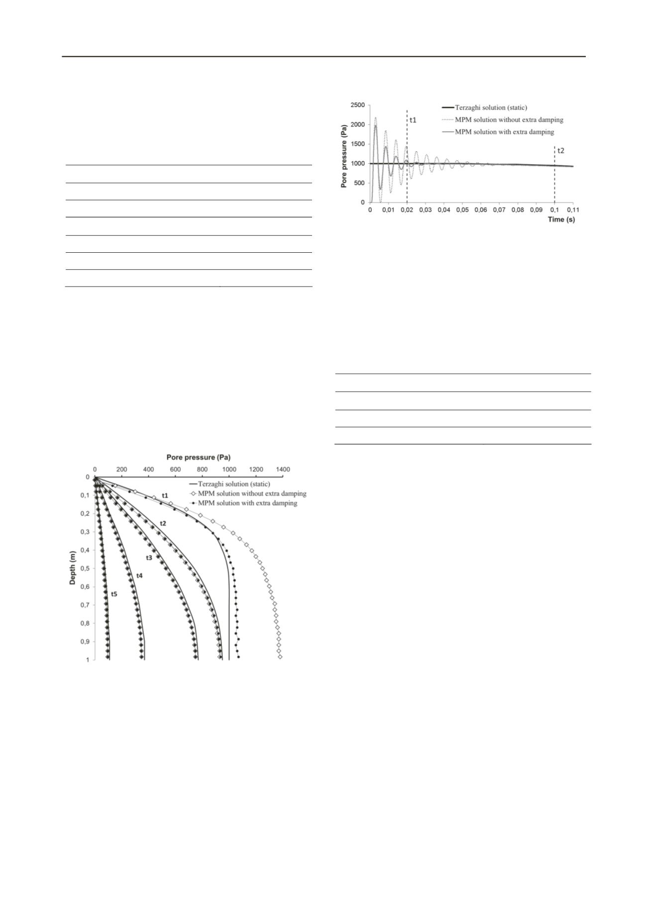
Figure 5 shows the evolution of the pore pressure along
depth at different times for both simulations. Figure 6 provides
the evolution of the pore pressure of the material point located
at the bottom of the sample. The numerical solution is naturally
damped in any case because of the coupling term of the hydro-
mechanical formulation, which is explained by water flow in
soil pores (at t
2
both MPM numerical solutions fit the static
solution). However, the implementation of viscous boundaries
(extra damping) is essential to damp the solution as quick as
possible if the aim is to capture the quasi-static equilibrium. At
t
1
(Fig. 5 and 6) the MPM solution with extra damping almost
adjusts the static solution while the MPM solution with fixed
boundary on the bottom still has a strong dynamic behavior.
Figure 5. Comparison of analytical and MPM solutions (with
and without extra damping on the bottom) for one-dimensional
consolidation at different times (t
1
=0.02s, t
2
=0.1s, t
3
=0.2s,
t
4
=0.5s, t
5
=1s).
4 SLOPE FAILURES
4.1
Simple case
Two plane strain theoretical cases are presented below. Both
simulations have been solved using a purely mechanical
formulation and they concern slope failures with the same initial
geometry and boundary conditions (the lowest boundary of the
model is fixed and horizontal displacements are restricted in the
lateral boundaries.
Figure 6. Evolution of the pore pressure for the deepest material
point.
The constitutive model used in both cases is the Mohr-
Coulomb criterion. The first case is characterized by a frictional
material, while the second is a cohesive material. In order to
initiate the failure of the slopes the strength parameters were
suddenly decreased. In the first simulation, the friction angle
has been reduced from 42º to 28º whereas the undrained
strength was reduced from 100kPa to 10kPa. Other common
material parameters are given in Table 3.
Table 3. Material parameters for the simulation of slope stability cases
Material parameter
Dry unit weight γ (kN/m
3
)
16
Young modulus E (MPa)
10
Poisson ratio ν
25
Figure 7a shows the initial particle distribution for both
simulations, and figures 7b and 7c show the two final
distributions after the failure. In both simulations large
deformations occur but the typology of the movement is
completely different. For the frictional material, a shallow
failure is developed and the main part of the movement occurs
during the first 50 seconds. On the contrary, the failure induced
for the cohesive material is deeper and in this case the time
elapsed to stabilize the slope is around 450 seconds.
This example shows the great importance of the strength
parameters and their evolution in the geometry and formation of
a failure. The method provides in a natural way the highly
deformed geometry of the slope after failure.
4.2
Aznalcóllar dam
The Aznalcóllar dam failure was described in Alonso & Gens
(2006). In a recent contribution, Zabala & Alonso (2011)
described an MPM analysis of the dam using a strain softening
constitutive model for the foundation soil.
A significant result of the analysis was an accurate
prediction of the geometry of the failure surface. Also the first
few meters of displacement after the instability where modeled.
A saturated porous media was considered and the hydro-
mechanical interactions were formulated in MPM. The model
was two-dimensional and a regular computational mesh was
used. A non-associated strain softening Mohr-Coulomb
constitutive law was implemented and calibrated for the clay
foundation. Figure 8 shows the development of the failure
surface preceding the final rupture. Figure 9 shows the
deformation of the mesh. The position of material points
provides a direct visual representation of the failure.


