859
Technical Committee 103 /
Comité technique 103
Proceedings of the 18
th
International Conference on Soil Mechanics and Geotechnical Engineering, Paris 2013
The stiffness of the thawed soil in the numerical analysis is
determined from Poisson’s ratio and the modulus which is
related to the coefficient of consolidation (Janbu 1970, Berntsen
1993). Some variables for “predefined fields” in Abaqus are
defined. The initial pore water pressure is set to zero. The initial
temperature of the frozen soil(ground temperature) in assumed
to be zero to compare the results with the simplified Neumann’s
solution in Eq. 2.The soil is also considered to be fully saturated
prior to thawing. Detailed procedures for defining “predefined
fields”, “initial conditions”, and thermal boundary conditions
are available in the Abaqus FEA.The analytical solution from
(Eq. 2) has been compared with the result obtained from a
numerical analysis using axisymmetric geometry and coupled
temperature-pore pressure elements in Abaqus. The thawing
depth from the numerical simulation is obtained by plotting the
time at which the temperature is changed from negative to
positive
) at selected nodes in the frozen soil layer. A very
good agreement is obtained from the analytical solution and
numerical simulation (see Figure 2).
2.2
Excess pore-water pressure
One of the consequences of spring thawing is that the frozen
water is melted upon thawing. Consequently, excess pore water
is generated depending on the overburden stress from the
pavement layers and external loading from the traffic. In the
case where a thick ice layer exists, an excess pore water
pressure can develop even from self-weight loading of the soil
lying on the ice layer. This phenomenon was modeled
analytically by Nixon(1973). The analysis is based on the
principle of heat conduction and Terzaghi’s one-dimensional
consolidation theory. From the coupled numerical analysis
(using Abaqus), it is possible to obtained excess-pore water
pressure. The amount of excess pore water pressure is very
sensitive the volumetric thermal expansion of pore water in the
voids of the frozen soil and the stiffness of the frozen soil. So, a
direct consideration of the output from the numerical analysis
may be misleading. Since we can accurately predict the
advancement of thawing by using the numerical analysis, we
can relate the development of excess pore water to the thawing
rate. A hydrostatic pore water pressure can be assumed for a
thawed soil if no additional loading exists. For example, for a
frozen subgrade soil under a pavement, the excess pore water
pressure will be the total overburden pressure (asphalt, base and
sub-base layers) including the loading from the traffic. This
assumption is valid for undrained conditions. In many cases,
subbase materials (aggregates) facilitate the dissipation of
excess pore water pressure. Then, post-thaw consolidation
follows. Detail analysis of one-dimensional thaw consolidation
is presented in Morgenstern and Nixon(1971).
2.3
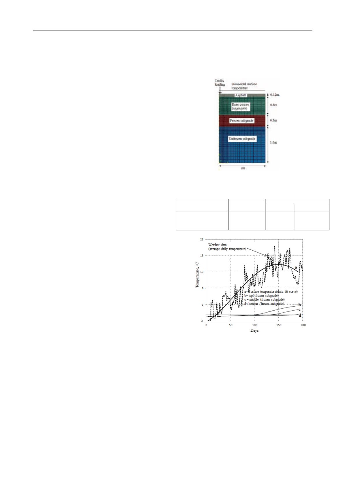
Modelling of thawing subgrades in pavements
Most of the analytical solutions available in the literature for
the thawing process are based on a one step temperature
increment on the surface. In reality, the change of surface
temperature is neither a step change nor constant. It is closer to
a sinusoidal curve. An advantage is gained by using numerical
analysis for different boundary conditions and pavement layers.
An axisymmetric geometry is modeled in Abaqus as shown in
Figure 3. This modeling(geometrically) is a reasonable
approximation for isotropic behavior of pavement materials and
an efficient computation time is obtained for the numerical
thermal analysis. The assumed thermal properties of the asphalt
materials and base course are listed in Table 2. The frozen
subgrade is modeled in the same way described in section 2.1.
A sinusoidal surface temperature is considered based on a local
weather data in Norway (Figure 4). The sinusoidal equation for
the temperature data is established. A Fourier transformation is
used to obtain the Fourier coefficients which are used as input
in Abaqus to provide a smooth increment of temperature for
each time increment.
Figure 3: Numerical model
Table 2: Thermal properties of the asphalt and base layers
Parameters
Unit
Value
Asphalt
Base-course
Conductivity
Specific heat
Coefficient of expansion
J/m.s.
0
C
J/kg.
0
C
/
0
C
0.75
920
2.2 x 10
-5
0.5
850
3 x 10
-6
Figure 4 Temperature variation during spring thawing
Assuming a uniform initial ground temperature Tg=-2
0
C the
temperature distribution in the frozen subgrade due to the
change of surface temperature on the pavement surface is
shown in Figure 4. It is noted that it takes about 90 days for the
frozen layer to start thawing from the time since the surface
temperature has been greater than
0℃
. Full scale field tests
(Nordal and Hansen 1987) showed a time period of 70 days for
the temperature measurement at 1.93m below the pavement
surface for the subgrade soil temperature to be changed from
negative to positive temperature(in degree celcius). Nordal and
Hansen measured the temperature variations at at depth of
0.05m, 0.15m, 0.63m, 0.93m and 1.93m. The measurements
showed that the surface temperature is higher than the data used
in our numerical analysis. In accounting this fact, the
approximation obtained from the numerical analysis can be
accounted for practical case studies.
The analytical solutions for temperature distributions (for
example Stephan’s formula) relate the thawing depth to be


