838
Proceedings of the 18
th
International Conference on Soil Mechanics and Geotechnical Engineering, Paris 2013
2.1 Static Load Test Pile Foundations
Currently static load test yield in the most reliable way to
determine the load capacity, but has some weakness i.e cost
and time-consuming. Poulos and Davis (1980) stated that one
of the usability of this test is its ability to compare between
static load limit bearing capacity obtained from the dynamic
and static formulas. Load test results in accordance with ASTM
D-1143 shown as a load-movement curve. Prakash and Sharma
(1990) described the full procedure for determining the limit
bearing capacity of static load test results with some methods of
interpretation.
2.3 Artificial Neural Network Model
Artificial Neural Network (ANN) is the information processing
system that has performance characteristics such as human
nerve network. Artificial neural network is a dynamic system (a
system that can be changed) as it can be trained and have the
ability to learn. Neural networks can work well even in the
presence of confounding factors such as uncertainty,
inaccuracy, and partial truth in the processed data (Fausett,
1994; Kurup and Dudani, 2002; Nugroho, 2003; Jeng et al.,
2005; Wang et al., 2005).
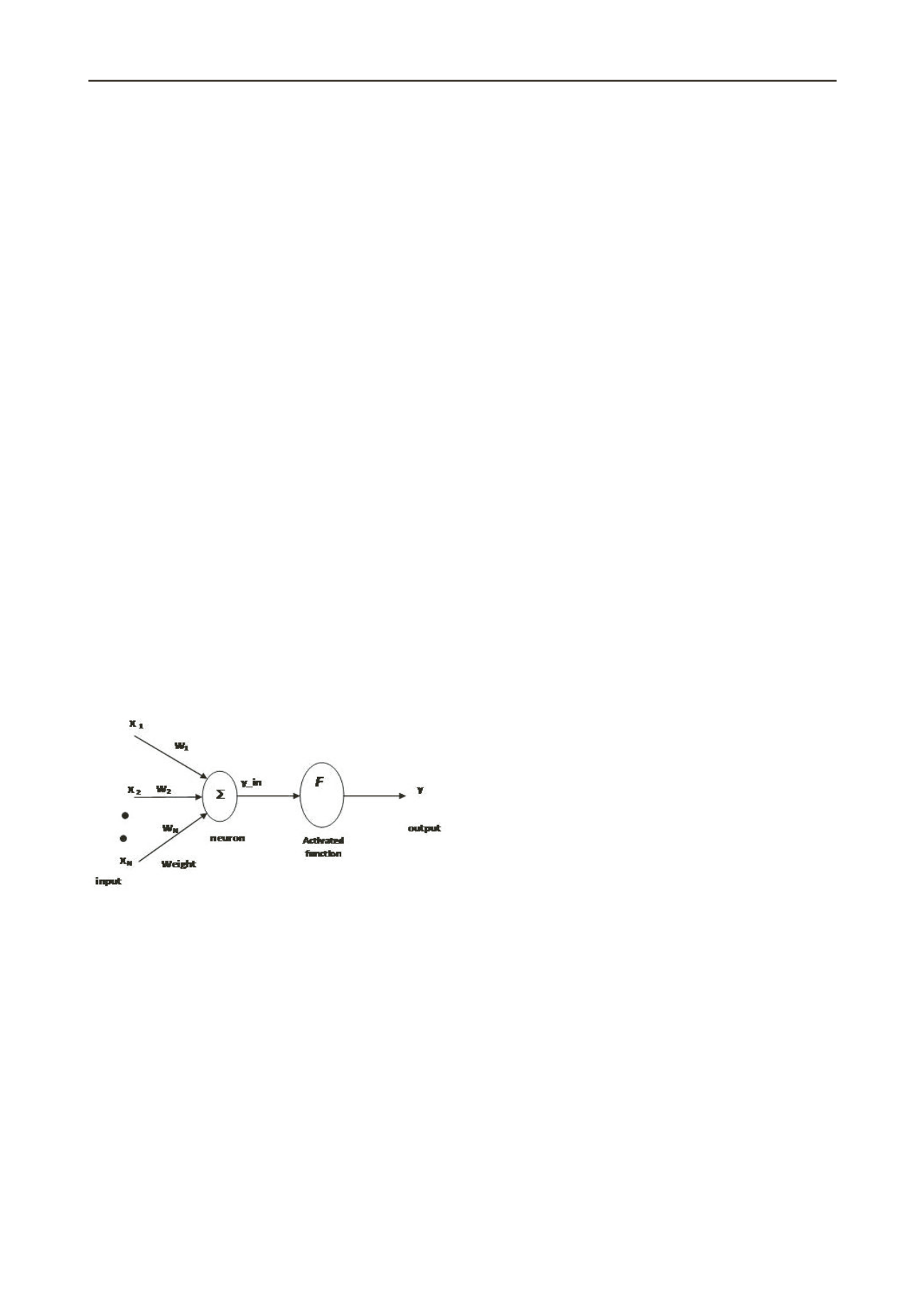
Neural network consists of several interconnected neurons.
Neurons transform information received via the connection to
the discharge of other neurons. On artificial neural networks,
this connection is called a weight. Information (input) is stored
at a particular value on the corresponding weights are then sent
to other neurons by the arrival of a certain weight. Input will be
processed by the propagation function that will sum the values
of all weights that come. The sum is then compared with a
threshold value, usually through an activation function of each
neuron. Neurons will be activated when the input is passed a
certain threshold value, but if not and vice versa. Neurons that
are activated will send the output via the output weights to all
the neurons connected with it. This process is described in
Figure 1 (Kusumadewi and Hartati, 2006).
Figure 1. Tipical of an Artificial Neural Network (Kusumadewi dan
Hartati, 2006)
Fausett (1994) and Kasabov (1998) classified models based
on artificial neural networks i.e. network architecture (single
layer, multi layer, competitive layer), presence or absence of
feedback connections (feed-forward networks and feedback
networks), the method of determining the connection
weights/training/ algorithm (unsupervised and supervised), and
activation function (Identity, Step Binary, Binary Sigmoid,
Sigmoid Bipolar).
2.3.1 Evaluation of Precision, Accuracy, and Robustness ANN
Modeling Results
Cooper and Emory (1997) in Somantri and Muhidin (2006)
defined the precision as a measure of how much something
means to give consistent results. Precision closely with a variety
of data, measured by the coefficient standard errors. The smaller
the standard error coefficient means higher precision. Accuracy
is how well an instrument measures what it is supposed to be
measured, therefore the level of accuracy is measured using the
average. The closer the value 1 (one) indicates the more
accurate.
3. RESEARCH METHODS
This study was conducted in several major stages i.e
preliminary, model development, model verification, and
calibration model. The resulting final model named NN_Qult.
In this study, the results of static load test was used as a
reference for measuring the precision and accuracy of modeling
results with the ANN approach. Some of the conventional
formulas (Meyerhof, 1976 and Briaud,1985 in Coduto, 1994)
were chosen for its performance compared with the results of
ANN modeling approaches.
3.1 Preliminary Phase
Data was collected from the Final Report of Investigations and
Axial Static Load Test Reports of load pile foundation. Datas
taken at several building projects on the Java Island that use
pile foundation.
To manufacture the artificial neural network model in this
study, there are several things that need to be considered such
as model input variable selection, data management, the
determination of the model architecture, network criteria
selected as the final model (Shahin et al.,2001). The selection
of the model input variables was based on a prior knowledge
(Maier and Dandy, 2000 in Shahin et al.,2001).
The available data was divided in to the proportion of 2/3
for the phase of training (i.e. training and testing) and 1/3 for the
validation phase (Hammerstrom ,1993 in Shahin et al.,2001).
Training set for adjusting the connection weights, testing set to
check the ability of the model in several variations of the
training phase, the validation set to estimate the ability of the
model that has passed through phases of training to be applied.
Another thing to note is the pattern of each sample data set used
for training and validation phases were expected to represent the
same population, then some random combination tried to obtain
some consistency in the statistical value of the mean, standard
deviation, minimum, maximum, range (Shahin et al., 2002b).
Because of the unavailability of the method for determining
the optimum architecture, so in this study, fixing the number of
hidden layers and choosing the number of nodes in each layer
were conducted. Determination of a network was selected and
some combinations of networks were trained. Observed output
and predicted output were compared qualitatively by looking at
a visual comparison of plot points of data and quantitative by
statistical parameters test.
3.2 Model Verification
Model verification was conducted by sensitivity analysis.
Sensitivity analysis is a method for extracting the influence of
the relationship between input variables with output variables
on the network. The first experiment with installing the first
input variable values vary between the mean values ± standard
deviation or between the minimum and maximum value while
the other input variables fixed at the mean value of each.
Similar experiments carried out at the other input variables. This
process will generate a graph the relationship between each
input variable versus network predicted output variables. The
strength of the final model assessed the suitability of the final
model with the existing theory (Shahin et al., 2002a; Samui and
Kumar, 2006).
3.3 Calibration Model
Sensitivity analysis phase produces the final model i.e
NN_Qult. The model was then tested with the full-scale static
load test as a validation. Some selected conventional formulas
were chosen and compared with the final model NN_Qult. The
tools used to perform comparison were a few statistic


