3011
Technical Committee 215 /
Comité technique 215
,
L L
L L
L t
nS
v
f
t
z
(4)
,
G G
G G
G t
nS
v
f
t
z
(5
)
where
ρ
G
and
ρ
L
are liquid density and gas density respectively,
n
is the porosity which is determined by
m
sd
and
ε
,
S
L
and
S
G
are
liquid saturation and gas saturation respectively,
v
L
and
v
G
(m/s)
are liquid velocity and gas velocity respectively.
Mechanical compression of MSW is expressed by the one-
dimensional compression model expressed as Eq.1. The
effective stress
σ’
is expressed as Bishop’s equation for
unsaturated soils (Bishop 1959).
Main governing equations of the BHM coupled model are
shown as Eqs.1-5.The BHM coupled model is numerically
solved by the finite difference method and Gauss-Newton
method.
Based on Chen et al. 2009 and Reddy et al. 2008, two
hypothetical waste samples with a height of 5m are studied for
MSWs in Qizishan landfill, China and Orchard Hills landfill,
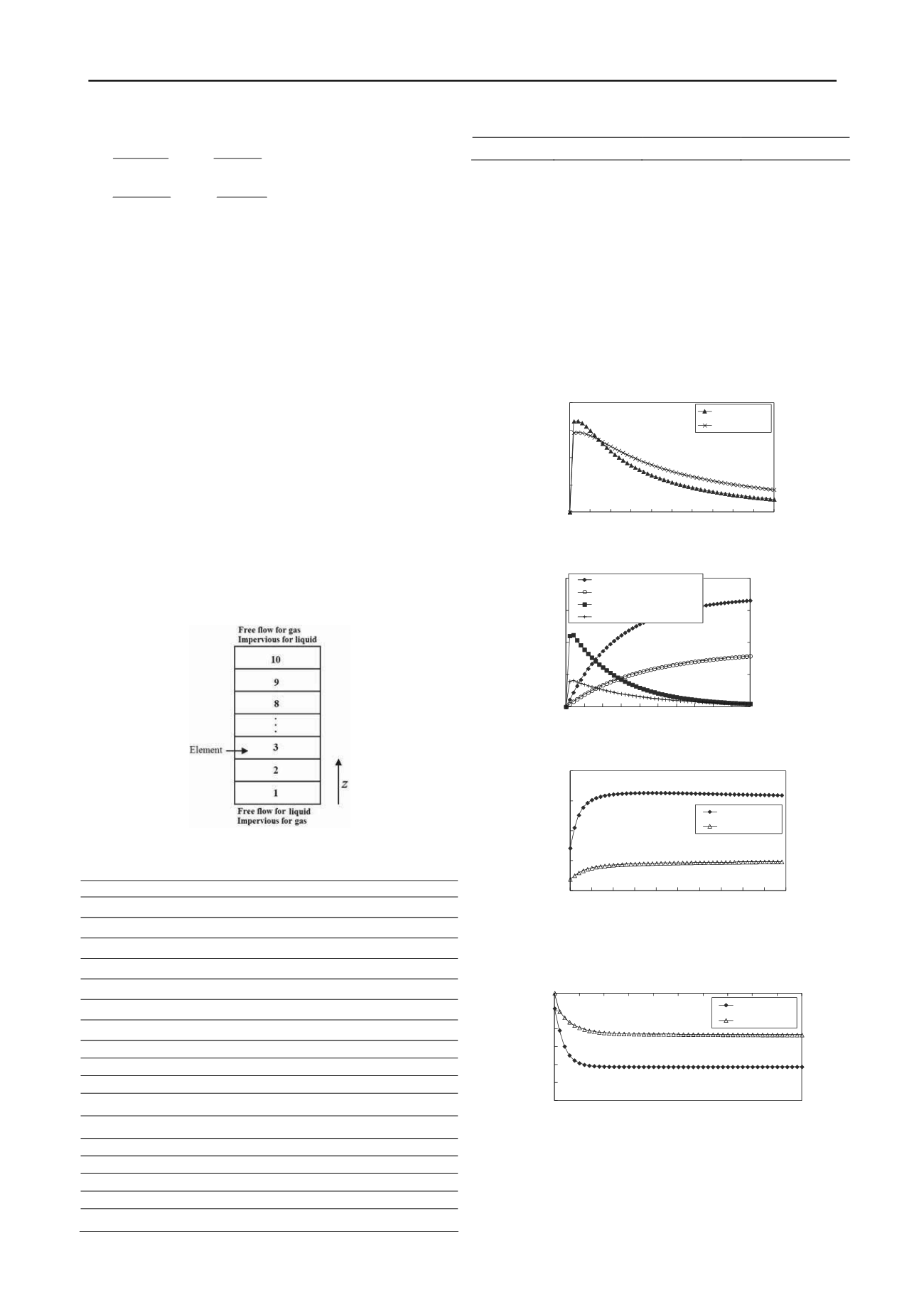
USA, respectively. As shown in Figure 4, top boundary is
impervious for liquid but free for gas flow, and the bottom
boundary is impervious for gas but free for liquid flow. The
total stress is set to be zero at the top boundary, and
compression strain is set to be zero at the bottom boundary.
Each element is 0.5m high, and the time step is 10
-5
day
-1
.
Parameters applied are shown in Table 2. Gas pressure,
leachate/gas production and settlement are analysed through the
BHM coupled model.
Figure 4. Schematic diagram of a hypothetical waste sample
Table 2. Parameters applied in the BHM coupled model
m
ds
1
/
m
s
0
m
ds
2
/
m
s
0
m
ds
3
/
m
s
0
w
0
(wet)
0.35*
0.20*
0.10*
0.60*
0.05
#
0.25
#
0.20
#
0.44
#
f
water
d
S
γ
0
(kN/m
3
)
e
0
1.0*
1.87*
7.5*
3.0*
1.0
#
0.85
#
5.0
#
1.4
#
C
C
’
C
C∞
’
σ
0
’
(kPa)
ε
tS
(
σ
0
’
)
0.25*
0.17*
10*
0.38*
0.28
#
0.17
#
10
#
0.20
#
m
vG
n
vG
α
vG
(m
-1
)
γ
vG
0.26*
#
1.35*
#
25.6*
#
3.0*
#
μ
L
(kgm
-1
s
-1
)
μ
G
(kgm
-1
s
-1
)
Mol
G
(kgmol
-1
)
R
(m
3
PaK
-1
mol
-1
)
1.0×10
-3
*
#
1.4×10
-5
*
#
0.03*
#
8.314472*
#
c
1
’
(day
-1
)
c
2
’
(day
-1
)
c
3
’
(day
-1
)
c
(day
-1
)
0.00023*
#
0.00013*
#
0.00003*
#
0.0016*
#
k
0
(m
2
)
θ
S
θ
r
η
10
-11
*
#
0.75*
#
0.035*
#
-0.11*
#
T
(K)
g
(ms
-2
)
ρ
L
(kgm
-3
)
P
a
(Pa)
303*
#
9.8*
#
994.13*
#
101320*
#
Note: * is for MSWs in Qizishan landfill, China
#
is for MSWs in Orchard Hills landfill, USA
As shown in Table 2, waste sample from Qizishan landfill
has higher organic content (i.e.
m
ds
1
which represents highly
degradable component) and initial moisture content (i.e.
w
0
),
compared to that from Orchard Hills landfill. Two samples are
both assumed to have an optimum biodegradation condition (i.e.
f
water
=1.0). Simulation results are shown in Figure 5-8. It
indicates that gas pressure of waste sample from Qizishan
landfill have larger gas pressure during the early stage. Gas
generation rate, gas production, leachate production and surface
settlement of waste sample from Qizishan landfill are all much
greater than that from Orchard Hills landfill.
0
400
800
1200
1600
0 5 10 15 20 25 30 35 40 45 50
Gas pressure
at thebottom (Pa)
Time(year)
Qizishan
OrchardHills
Figure 5. Gas pressure at the bottom of waste samples
0.00
0.01
0.02
0.03
0.04
0.0
0.1
0.2
0.3
0.4
0 5 10 15 20 25 30 35 40 45 50
Gas generationrate
(m
3
kg
-1
year
-1
, dry basis)
Gas production
(m
3
kg
-1
, dry basis)
Time(year)
Left axis-Qizishan
Left axis-OrchardHills
Right axis-Qizishan
Right axis-Orchard Hills
Figure 6. Gas generation rate and gas production of waste samples
0
0.05
0.1
0.15
0.2
0 5 10 15 20 25 30 35 40 45 50
Leachateproduction(m
3
/m
3
)
Time(year)
Qizishan
OrchardHills
Figure 7. Leachate production per volume of waste samples
0.0
0.5
1.0
1.5
2.0
2.5
3.0
0 5 10 15 20 25 30 35 40 45 50
Settlement(m)
Time(year)
Qizishan
OrchardHills
Figure 8. Settlement of waste samples


