2805
Technical Committee 212 /
Comité technique 212
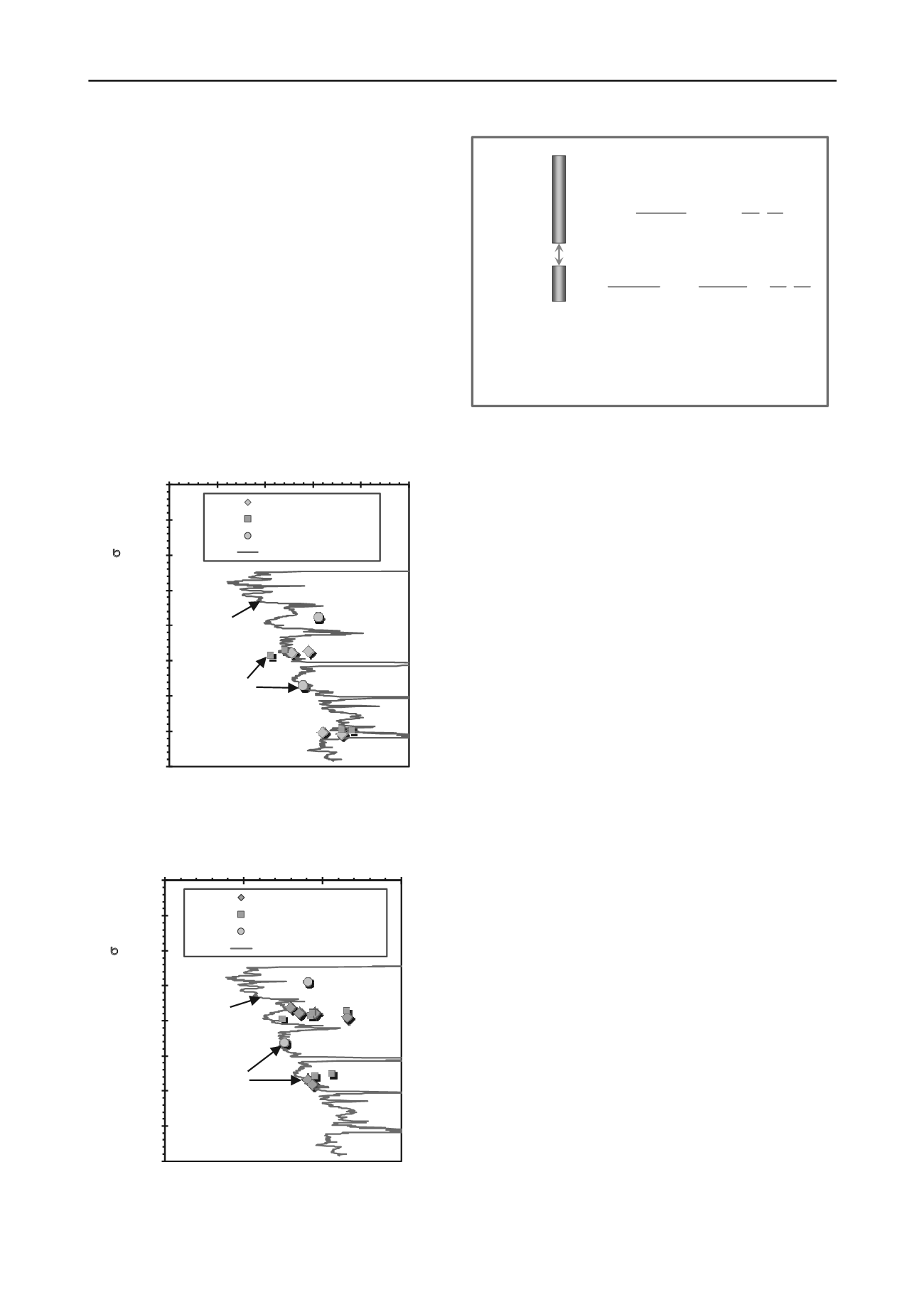
O-Cell Elastic Continuum Solution
01
1
1
1 1o1s
1
r
L 2
wrG
P
P = applied force
L = pile segment length
r
o
= pile shaft radius
G
s
= soil shear modulus along sides
G
sb
= soil modulus below pile base
2o
2
2
2 2o2s
2
r
L 2
) 1(
4
wrG
P
Lower rigid segment in downward loading
Rigid pile segment under upward loading
upper
segment
(length L
1
)
lower
segment
(length L
2
)
O-Cell
w = pile displacement
= Poisson's ratio of soil
= G
s2
/G
sb
(Note: floating pile:
= 1)
= ln(r
m
/r
o
) = zone of influence
r
m
= L{0.25 +
[2.5 (1-
) – 0.25]}
P
1
= P
2
Base
f
p
≈ K
0
∙
vo
'
∙
tan
'
(5)
For soils with stress history of virgin loading-unloading, the
geostatic lateral stress coefficient can be evaluated from:
K
0
= (1-sin
')
∙
OCR
sin
'
(6)
In consideration of pile material type and method of installation,
the expression is modified to:
f
p
≈ C
M
∙
C
K
∙
K
0
∙
vo
'
∙
tan
'
(7)
where C
M
= interface roughness factor (= 1 for bored cast-in-
place concrete, 0.9 prestressed concrete, 0.8 for timber, and 0.7
for rusty steel piles) and C
K
= installation factor (= 1.1 for
driven piles; 0.9 for bored piles).
Calculated values of pile side friction are shown in Figure 3
and vary between 150 < f
p
< 250 kPa. These are comparable in
magnitude, and in some cases less than f
b
determined from the
O-cell load test series.
0
50
100
150
200
250
300
350
400
0
1
2
3
4
5
Effective Stress at Base,
vo
' (kPa)
Unit End Bearing, q
b
(MPa)
Mount Pleasant
Charleston
Drum Island
qb from CPTu
O-Cells
CPTu
Figure 2. Measured and calculated unit end bearing resistances
0
50
100
150
0
100
200
300
ddepth,
vo
' (kPa)
Unit Side Resistance, f
p
(kPa)
200
250
300
350
400
Effective Stress at Mi
Mount Pleasant
Charleston
Drum Island
fp from CPTu
O-Cells
CPTu
Figure 3. Measured and calculated unit side friction resistances
Figure 4. Elastic continuum solution for O-cell loading of piles
4.2.
Axial Pile Displacements
The elastic continuum solutions for an axial pile foundation are
detailed by Randolph and Wroth (1978, 1979) and Fleming et
al. (1992) by coupling a pile shaft with a circular plate. This can
be deconvoluted back into the separate components to represent
the original O-cell arrangement or into stacked pile segments
for a mid-shaft O-cell as well as for multi- staged O-cell setups.
For the simple case of rigid pile segments, Figure 4 presents the
elastic solution for a mid-section O-cell framework.
The stiffness of the surrounding soil is represented by a
shear modulus (G). The initial fundamental small-strain shear
modulus of the ground is obtained from the shear wave velocity
measurements:
G
0
=
T
∙
V
s
2
(8)
where
T
= total mass density of the soil. This small-strain
stiffness is within the true elastic region of soil corresponding to
nondestructive loading. To approximately account for non-
linearity of the stress-strain-strength behavior of soils, a
modified hyperbola is adopted (Fahey, 1998):
G = G
0
∙
[1 - (P/P
ult
)
g
]
(9)
where P = applied force, P
ult
= axial capacity of the pile
segment, and the exponent "g" is a fitting parameter (Mayne,
2007a, 2007b). Thus when P = 0, initially G = G
0
and at all
higher load levels the shear modulus reduces accordingly.
Data from monotonic loading in resonant column, torsional
shear, and triaxial shear tests with local strain measurements on
both clays and sands under drained and undrained conditions
have been compiled to evaluate the nonlinear modulus trends. A
summary of these data for a wide variety of soils has been
compiled and presented in Figure 5 (Mayne 2007b). The y-axis
(G/G
0
) can be considered as a modulus reduction factor to apply
to the measured small-strain stiffness attained from (8) using
site-specific V
s
field data. The x-axis (q/q
max
= 1/FS) is a
measure of the mobilized strength and can be considered as the
reciprocal of the factor of safety (FS) corresponding to the load
level relative to full capacity. In the case of pile capacity, the
mobilized strength is obtained from the ratio of applied load to
capacity (P/P
ult
= 1/FS)
The modified hyperbola given by (9) is also presented in
Figure 5 and can be seen to take on values of "g" exponent
ranging from 0.2 (low) to 0.5 (high) when compared to the lab
data. Usually, a representative exponent value g = 0.3 has been


