1964
Proceedings of the 18
th
International Conference on Soil Mechanics and Geotechnical Engineering, Paris 2013
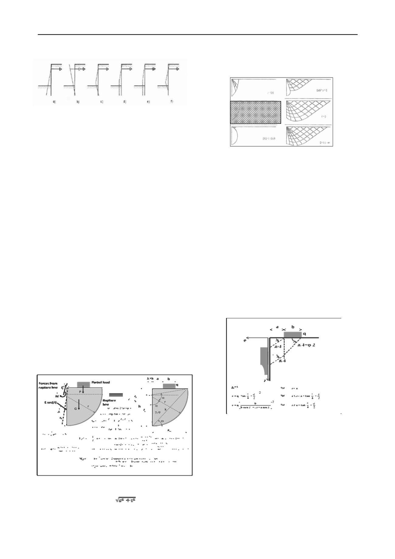
Figure 1,
A
nchored wall in failure composed of one or more rigid
segments connected by yield hinges in failure. This paper deals with
failure mode a) marked with rectangular.
A pressure jump near the top is then applied to ensure that the
effect of the distribution (in terms of total force and moment)
corresponds with the rupture figure The method has been
described in detail by Mortensen & Steenfelt (2001) and results
of calculated examples are compared with FE calculations.
3
COMPUTER PROGRAM ‘SPOOKS’
Although J. B. Hansen has developed a complete set of
diagrams to find the values of
K,
the earth pressure calculation
for a specific design situation is rather time consuming. To this
end GEO-Danish Geotechnical Institute has made a
commercially available computer program named ‘SPOOKS’.
Here, apart from the geometry of the excavation, the soil
conditions and water tables, only a selection of the total wall
movements (as shown in Figure 1) is necessary as input. The
results are a distribution of both earth and water pressures,
curve of bending moments along the wall, tip level, and anchor
force. All together ready for the final design of the sheet pile
wall profile and anchor. However, this program has no facility
to include a partial surface load.
4
THEORY OF PLASTICITY
A method to assess the extra soil pressure caused by a partial
load has been introduced by J.S. Steenfelt and B. Hansen
(1984). The Danish method to calculate the earth pressure
coefficient from a relevant rupture line has been adopted. A
circular rupture line is used as an appropriate choice for a
rotation about a point at the anchor level. The stresses from the
rupture line are determined by the Kötter’s differential equation.
The total force is found by integration of this equation presented
by Brinch Hansen (1953) and shown as the resulting force (
F
o
)
and moment (
M
o
) about the centre of the circle as shown in
Figure 2 where the significance of the variables is indicated.
Figure 2, Analytical method where circular rupture figure is applied.
Negative values of
φ
and
δ
shall be applied as the rupture is active.
It should be mentioned that
t
c
=
where
t
c
refers to the
starting point of the integration where the rupture circle meets
the soil surface and
σ
and
τ
are coordinates to the yield point in
the Mohr’s circle. The function
q(
λ
)
refers to the value of
q
in
the point where the circle meets the surface. (
q
beneath the load
and 0 otherwise). The three unknowns (
λ
,
E
, and
z
p
) are finally
found by the three equilibrium equations.
Figure 3, Rupture figures with different rotation points (
ρ:
relative
height from the bottom of the wall). The figures are drawn for
φ
= 30°,
c
= 0 and rough wall rotating clockwise. The pure line rupture is
investigated analytically in this paper (shaded in the figure).
This method (Figure 3 shaded) is in detail introduced and
discussed by the authors and the results of a large number of
load scenarios are presented in their paper.
5
EMPIRICAL METHOD
It is usual practice to apply a soil pressure derived from the
distribution for the uniformly loaded surface. A minor part of
this distribution is then used situated to a depth interval defined
by inclined lines through the soil.
In Figure 4 a method of this kind often used in Denmark is
shown. However, a tail below the lower line has been in this
method proposed by K. Mortensen (1973) who has pointed out
the complexity of the problem assuming a smooth wall that
rotates anti-clockwise about a point below the tip of the wall.
Consequently, the upper part with the even distribution is given
by an active Rankine rupture figure. The tail is probably
inspired by calculations by Coulomb’s method where the lower
part is more dependent of other parameters than
a
and
b.
Figure 4, Empirical method based partly on the Coulomb’s earth
pressure theory.
As this method is often used also for other movements, en lieu
of other procedures it is adopted here as an example of an
empirical solution.
6
ELASTIC SOLUTION
An elastic solution developed by Boussinesq (1885) is often
used because of its simplicity as shown in Figure 5. Besides the
theory of elasticity a smooth vertical wall without any
movement is assumed. This method is often questioned as the
resulting distribution is too large and situated much too high on
the wall with respect to results from model tests and
calculations based on the Coulomb’s method.


