1965
Technical Committee 207 /
Comité technique 207
This is also the authors experience when the movement of
the wall is anti clockwise about a low point in the wall.
However, if the movement is a clockwise rotation about the
anchor (as in this paper) the assumptions for an elastic solution
are more justified.
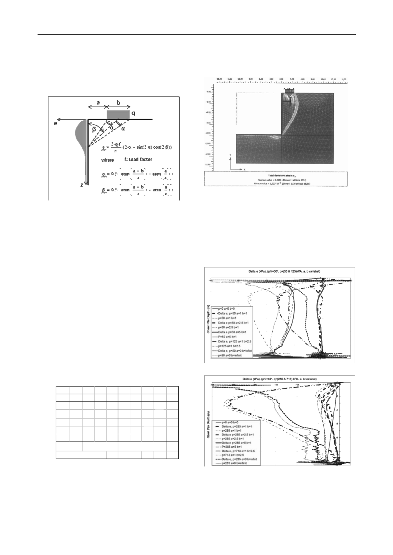
Figure 5, Elastic solution by Boussinesq (1885)
7
FINITE ELEMENT METHOD
In order to validate the method a number of load scenarios have
been calculated by the FE program Plaxis 2011.
A 2D mesh pattern has been generated using triangular finite
elements (15-noded). Sand is modeled in drained conditions
using the Mohr-Coulomb constitutive model. The sheet pile
wall is assumed weightless and with a large stiffness to prevent
any interaction of stresses caused by deformation of the wall.
The initial geostatic conditions are calculated first. Mesh
sensitivity analyses have been carried out and an optimal mesh
pattern with respect to element size and obtained accuracy has
been chosen for the final analyses.
Plaxis plastic analyses (small deformation theory) and
Updated Mesh (large deformation theory) have been applied to
estimate the effect of the wall movement on the results. The
calculations are carried out in different ways considering the
impact the staged construction (excavating after, before or at the
same time with the load application) has on the results.
Some different load scenarios are modeled and calculated to
illustrate the problem. The loads / pressures applied over the
foundations are chosen in such a way that the foundation
bearing capacity is satisfied. The load scenarios are shown in
Table 1.
Table 1, Load scenarios calculated
A unit weight has been applied to the soil to provide a realistic
stress distribution near the top of the wall. Interface elements
are applied along the wall. However, the soil strength at the
interface has not been reduced as a rough wall is considered.
The influence of the load on the wall has thus been derived as
the difference between results of calculations of the wall with
load and unit weight and with unit weight alone.
A rigid anchor is applied at a depth corresponding to 0.8*h
referring to the bottom of excavation or the height of the wall h.
The anchor point ensures a rotation around this point during
failure (Figure 6).
Figure 6 FE model example, (
φ
=30◦
a
=1.0 m
b
=2.5 m or
a
/
b
=0.4
p
=125
kPa).
A complete presentation of the results is not included due to
lack of space. The normal pressure (
e
) on wall from the soil, and
the soil plus load, and the additional pressure from the load
derived as their difference (Delta
e
) are derived from the
interface zone as given in Figure 7 and 8 for both soil types
considered. The FE results are used as benchmarks for the
accuracy of the other methods and shown relative to those in the
discussion.
Figure 7 FE models results (
φ
=30◦)
No
φ
a b q No
φ
a b q
(deg) (m) (m) (kPa)
(deg) (m) (m) (kPa)
1 30 1 3 125 6 40 1 3 71
2 30 1 1 50 7 40 1 1 28
3 30 3 1 50 8 40 3 1 28
4 30 5 1 50 9 40 5 1 28
5 30 0
∞
50 10 40 0
∞
285
h = 12 m γ = 14 kN/m
3
c = 0 kPa rough wall
Height to rotation point:
h
ρ
= 9.6 m
3
5
5
5
2.5
2.5
2.5
2.5
Figure 8 FE models results (
φ
=40◦)
8
DISCUSSION OF CALCULATIONS
It was expected that a study of the theory of plasticity would
yield a deeper insight into the problem and provide useful
results. However, our calculations have produced rather
scattered results. The calculations presented by Steenfelt &
Hansen do by no means suggest simple relations to the input


