799
Technical Committee 103 /
Comité technique 103
nonhomogeneous soil of dense strata with a weak layer
above. Also, in non-homogeneous soil, when the pile toe is
located in weak strata with a dense layer above, the
influence zone extends to 4
D
below and 2
D
above pile toe.
In homogeneous soil, however, the influence zone extends
to 4
D
below and 4
D
above pile toe.
Both measurements of cone point resistance and sleeve
friction are incorporated as model inputs. This allows the
soil type (classification) to be implicitly considered in the
RNN model.
Several CPT tests used in this work include mechanical
rather than electric CPT data and thus, it was necessary to
convert the mechanical CPT readings into equivalent
electric CPT values as the electric CPT is the one that is
commonly used at present. This is carried out for the cone
point resistance using the following correlation proposed by
Kulhawy and Mayne (1990):
19.1
47.0
Mechanical
a
c
Electric
a
c
p
q
p
q
(1)
For the cone sleeve friction, the mechanical cone gives
higher reading than the electric cone in all soils with a ratio
in sands of about 2, and 2.5–3.5 for clays (Kulhawy and
Mayne 1990). In the current work, a ratio of 2 is used for
sands and 3 for clays.
3.2
Data division and preprocessing
The next step in the development of the RNN model is dividing
the available data into their subsets. In this work, the data were
randomly divided into two sets: a training set for model
calibration and an independent validation set for model
verification. In total, 20 in-situ pile load tests were used for
model training and 3 tests for model validation. A summary of
the tests used in the training and validation sets is not given due
to the lack of space. Once the available data are divided into
their subsets, the input and output variables are preprocessed; in
this step the variables were scaled between 0.0 and 1.0 to
eliminate their dimensions and to ensure that all variables
receive equal attention during training.
3.3
Network architecture and internal parameters
Following the data division and the preprocessing, the optimum
model architecture (i.e., the number of hidden layers and the
corresponding number of hidden nodes) must be determined. It
should be noted that a network with one hidden layer can
approximate any continuous function if sufficient connection
weights are used (Hornik et al. 1989). Therefore, one hidden
layer was used in the current study. The optimal number of
hidden nodes was obtained by a trial-and-error approach in
which the network was trained with a set of random initial
weights and a fixed learning rate of 0.1; a momentum term of
0.1; a tanh transfer function in the hidden layer nodes; and a
sigmoidal transfer function in the output layer nodes. The
following number of hidden layer nodes were then utilized: 2, 4,
6, …, and (2
I
+1), where
I
is the number of input variables. It
should be noted that (2
I
+1) is the upper limit for the number of
hidden layer nodes needed to map any continuous function for a
network with
I
inputs, as discussed by Caudill (1988). To obtain
the optimum number of hidden layer nodes, it is important to
strike a balance between having sufficient free parameters
(connection weights) to enable representation of the function to
be approximated and not having too many, so as to avoid
overtraining (Shahin and Indraratna 2006).
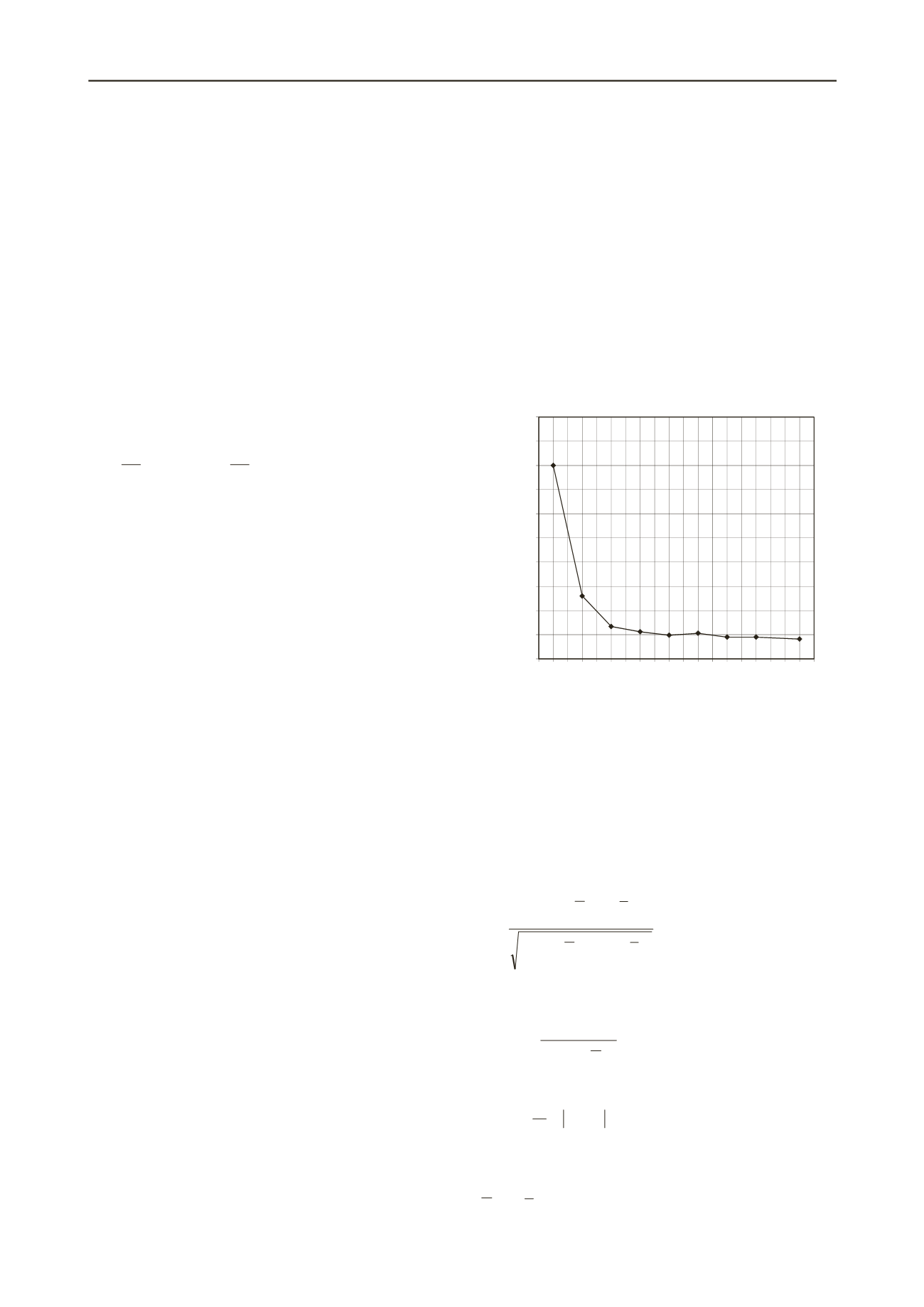
To determine the criterion that should be used to terminate
the training process, the normalized mean squared error
between the actual and predicted values of all outputs over all
patterns is monitored until no significant improvement in the
error occurs. This was achieved at approximately 10,000
training cycles (epochs). Figure 3 shows the impact of the
number of hidden layer nodes on the performance of the RNN
model. It can be seen that the RNN model improves with
increasing numbers of hidden layer nodes; however, there is
little additional impact on the predictive ability of the model
beyond 8 hidden layer nodes. Figure 3 also shows that the
network with 19 hidden layer nodes has the lowest prediction
error; however, the network with 8 hidden nodes can be
considered optimal: its prediction error is not far from that of
the network with 19 hidden nodes, and it has fewer connection
weights and is thus less complex. As a result of training, the
optimal network produced 9 × 8 weights and 8 bias values
connecting the input layer to the hidden layer and 8 × 8 weights
and one bias value connecting the hidden layer to the output
layer.
0
5
10
15
20
25
30
35
40
45
50
1 2 3 4 5 6 7 8 9 10 11 12 13 14 15 16 17 18 19 20
Normalized MSE (× E�5)
No. hidden nodes
Figure 3. Effect of number of hidden nodes on RNN performance.
3.4
Model performance and validation
The performance of the optimum RNN model in the training
and validations sets is given numerically in Table 1. It can be
seen that three different standard performance measures are
used, including the coefficient of correlation,
r
, the coefficient
of determination (or efficiency),
R
2
, and the mean absolute
error, MAE. The formulas of these three measures are as
follows:
N
i
i
N
i
i
i
N
i
i
PP OO
PPOO
r
1
2
1
2
1
)
( )
(
)
()
(
(2)
N
i
i
N
i
i
i
OO
PO
R
1
2
1
2
2
)
(
)
(
1
(3)
N
i
i
i
PO
N
MAE
1
1
(4)
where
N
is the number of data points presented to the model;
O
i
and
P
i
are the observed and predicted outputs, respectively; and
O
and
P
are the mean of the predicted and observed outputs,
respectively.


