798
Proceedings of the 18
th
International Conference on Soil Mechanics and Geotechnical Engineering, Paris 2013
algorithm (Rumelhart et al. 1986). A comprehensive description
of backpropagation MLPs is beyond the scope of this paper but
can be found in Fausett (1994). The typical MLP consists of a
number of processing elements or nodes that are arranged in
layers: an input layer; an output layer; and one or more
intermediate layers called hidden layers. Each processing
element in a specific layer is linked to the processing element of
the other layers via weighted connections. The input from each
processing element in the previous layer is multiplied by an
adjustable connection weight. The weighted inputs are summed
at each processing element, and a threshold value (or bias) is
either added or subtracted. The combined input is then passed
through a nonlinear transfer function (e.g. sigmoidal or tanh
function) to produce the output of the processing element. The
output of one processing element provides the input to the
processing elements in the next layer. The propagation of
information in MLPs starts at the input layer, where the network
is presented with a pattern of measured input data and the
corresponding measured outputs. The outputs of the network are
compared with the measured outputs, and an error is calculated.
This error is used with a learning rule to adjust the connection
weights to minimize the prediction error. The above procedure
is repeated with presentation of new input and output data until
some stopping criterion is met. Using the above procedure, the
network can obtain a set of weights that produces input-output
mapping with the smallest possible error. This process is called
“training” or “learning”, which once has been successful, the
performance of the trained model has to be verified using an
independent validation set.
In simulations of the typical non-linear response of pile load-
settlement curves, the current state of load and settlement
governs the next state of load and settlement; thus, a recurrent
neural network (RNN) is recommended. A recurrent neural
network proposed by Jordan (1986) implies an extension of the
MLPs with current-state units, which are processing elements
that remember past activity (i.e. memory units). The neural
network then has two sets of input neurons: plan units and
current-state units (Figure 1). At the beginning of the training
process, the first pattern of input data is presented to the plan
units while the current-state units are set to zero. As mentioned
earlier, the training proceeds, and the first output pattern of the
network is produced. This output is copied back to the current-
state units for the next input pattern of data.
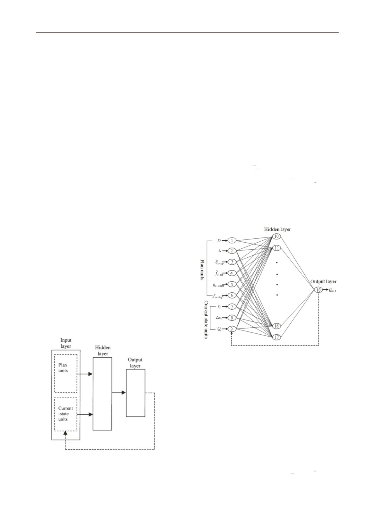
Figure 1. Schematic diagram of the recurrent neural network.
3. DEVELOPMENT OF NEURAL NETWORK MODEL
In this work, the RNN model was developed with the computer-
based software package Neuroshell 2, release 4.2 (Ward 2007).
The data used to calibrate and validate the model were obtained
from the literature and included a series of 23 in-situ full-scale
load-settlement tests reported by Eslami (1996). The tests were
conducted on sites of different soil types and geotechnical
conditions, ranging from cohesive clays to cohesionless sands.
The pile load tests include compression and tension loading
conducted on steel driven piles of different shapes (i.e., circular
with closed toe and H-pile with open toe). The piles ranged in
diameter between 273 and 660 mm with embedment lengths
between 9.2 and 34.3 m.
3.1
Model inputs and outputs
Six factors affecting the capacity of driven piles were presented
to the plan units of the RNN as potential model input variables
(Figure 2). These include the pile diameter,
D
(the equivalent
diameter is rather used in case of H-pile as: pile perimeter/π),
embedment length,
L
, weighted average cone point resistance
over pile tip failure zone,
tip c
q
, weighted average sleeve friction
over pile tip failure zone,
tip s
f
, weighted average cone point
resistance over pile embedment length,
shaft
c
q
, and weighted
average sleeve friction over pile embedment length,
shaft
s
f
. The
current state units of the neural network were represented by
three input variables: the axial strain,
ia
ε
,
, (= pile
settlement/pile diameter), the axial strain increment,
ia
ε
,
, and
pile load,
Q
i
. The single model output variable is the pile load at
the next state of loading,
Q
i
+1
.
Figure 2. Architecture of the developed recurrent neural network.
In this study, an axial strain increment that increases by
0.05% was used, in which
a
ε
= (0.1, 0.15, 0.2, …, 1.0, 1.05,
1.1, …) were utilized. As recommended by Penumadu and
Zhao (1999), using varying strain increment values results in
good modeling capability without the need for a large size
training data. Because the data points needed for the RNN
model development were not recorded at the above strain
increments in the original pile load-settlement tests, the load-
settlement curves were digitized to obtain the required data
points. This was carried out using Microcal Origin version 6.0
(Microcal 1999) and then implementing the cubic spline
interpolation (Press et al. 1992). A range between 14 to 28
training patterns was used in representing a single pile load-
settlement test, depending on the maximum strain values
available for each test.
It should be noted that the following aspects were applied
to the input and output variables used in the RNN model:
The pile tip failure zone over which
tip c
q
and
tip s
f
were
calculated is taken in accordance with Eslami (1996), in
which the influence zone extends to 4
D
below and 8
D
above pile toe when the pile toe is located in


