3504
Proceedings of the 18
th
International Conference on Soil Mechanics and Geotechnical Engineering, Paris 2013
the proposed theoretical model, representing the sea wave
actions exerted over the structure as boundary conditions.
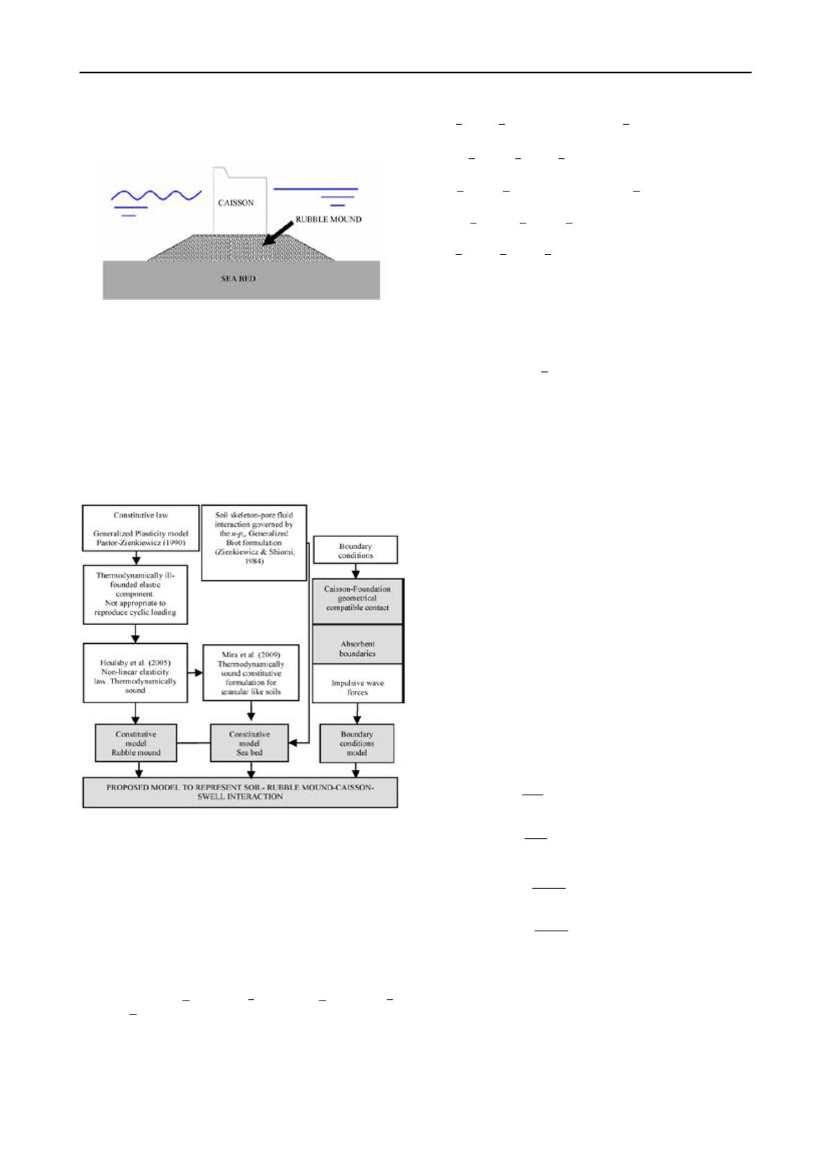
Figure 1. Physical systems involved in the soil-water-breakwater model
The theoretical model for the soil-water-breakwater
interaction proposed is developed in two dimensions under
plain strain idealization.
Once the sea bed, rubble mound and caisson governing
equations are derived, including the couplings involved as well
as the initial and boundary conditions, the theoretical model for
the soil-water-breakwater interaction proposed will be set.
In following figure (Figure 2), the main parts of the
theoretical model proposed in order to analyze the complex
seafloor-rubble
mound-caisson-swell
interaction
are
schematically shown. The novel theoretical contributions appear
in this figure over a dark colour box.
Figure 2. Outline of the proposed theoretical model
3 FINITE ELEMENT APROXIMATION
Once the kinematic relations as well as the constitutive laws are
integrated in the balance equations, a system of five partial
differential equations with five field variables is established.
The field variables involved are: sea bed skeleton displacement
sb
u
and pore water pressure
sb
w
p
, rubble mound skeleton
displacement
rm
u
and pore water pressure
rm
w
p
and caisson
displacement
ca
u
. The system of partial differential equations
can be discretized using standard Galerkin techniques
(Zienkiewicz et al 1999). After spatial discretization of the field
variables,
≅
sb
u sb
u N u
,
≅
sb
p sb
w
w
p
N p
,
≅
rm
u rm
u N u
,
≅
rm
p rm
w
w
p
N p
,
≅
ca
u ca
u N u
, the second order ordinary differential equation
system
(1)
-
(3)
is obtained (Stickle 2010)
(
)
T
1
2
T
sb
sb sb
sb sb
sb
sb
sb sb
sb
w
sb
sb
sb sb
sb sb
sb
w
w
d
Ω
+
+
Ω −
=
′
+
+
=
−
−
∫
σ
0
0
M u C u B
Q p
Q u H p S p
f
f
(1)
(
)
T
1
T
2
rm
rm rm rm rm
rm rm rm rm
rm
w
rm rm
rm rm rm rm
rm
w
w
d
Ω
′
+
+
Ω −
=
+
+
=
−
−
∫
σ
0
0
M u C u B
Q p
Q u H p S p
f
f
(2)
ca ca
ca ca
ca ca
ca
+
=
+
−
0
M u C u K u
f
(3)
Where
u
=
B SN
and
( )
( )
(
)
(
)
(
)
T
T
1
1
2
3
2
T
T
sb
sb
w
sb
sb
pw
sb
sb
u
sb
u
sb
sb
sb
imp
r
sb
sb
r
sb
sb
p
p
sb sb
sb
sb
w
p
imp
d
d
d
d
ρ
ρ
Ω
Γ
Ω
Γ
Ω +
Γ +
= + +
=
= ∇
Ω +
Γ
∫
∫
∫
∫
t
t
N
k
N b
t
R R R u
f
f
N
b
N q
(4)
( )
( )
(
)
(
)
T
T
1
2
T
T
rm
rm
w
rm
pw
rm
rm
rm
u
rm
u
rm rm rm
imp
c
rm
rm
rm rm
rm rm
w
imp
p
p
p
d
d
d
d
ρ
ρ
Ω
Γ
Ω
Γ
Ω +
Γ +
=
= ∇
Ω +
Γ
∫
∫
∫
∫
t
t
k
N b
N t
f
f
N
b
N q
(5)
(
)
(
)
T
T
ca
ca
ca
ca
ca
ca
ca
ca
imp
c
u
u
d
d
ρ
Ω
Γ
Ω +
Γ +
=
∫
∫
t
t
N b
N t
f
(6)
The matrices given in the system (1)-(3) are defined by
( )
( )
( )
T
T
T
ρ
ρ
ρ
Ω
Ω
Ω
=
Ω
=
Ω
=
Ω
∫
∫
∫
sb
rm
ca
sb
u
sb u
sb
rm
u
rm u
rm
ca
u
ca u
ca
d
d
d
M N N
M N N
M N N
(7)
T
T
,
Ω
Ω
=
Ω =
Ω
∫
∫
sb
rm
sb
p
sb
rm
p
rm
d
d
Q B mN Q B mN
(8)
( )
( )
( )
( )
T
T
1
1
Ω
Ω
=
Ω
=
Ω
∫
∫
sb
rm
sb
p
p
sb
sb
rm
p
p
rm
rm
d
Q
d
Q
S
N N
S
N
N
(9)
(
)
(
)
(
)
(
)
T
T
ρ
ρ
Ω
Ω
= ∇
∇ Ω
⋅
= ∇
∇ Ω
⋅
∫
∫
k
k
sb
rm
sb
sb
p
p
sb
w
rm
rm
p
p
rm
w
d
g
d
g
H N
N
H
N
N
(10)
α
β
α
β
α
β
=
+
=
+
=
+
sb
sb
sb
sb sb
rm
rm rm
rm rm
ca
ca
ca
ca ca
C M K
C M K
C M K
(11)


