3393
Technical Committee 307 + 212 /
Comité technique 307 + 212
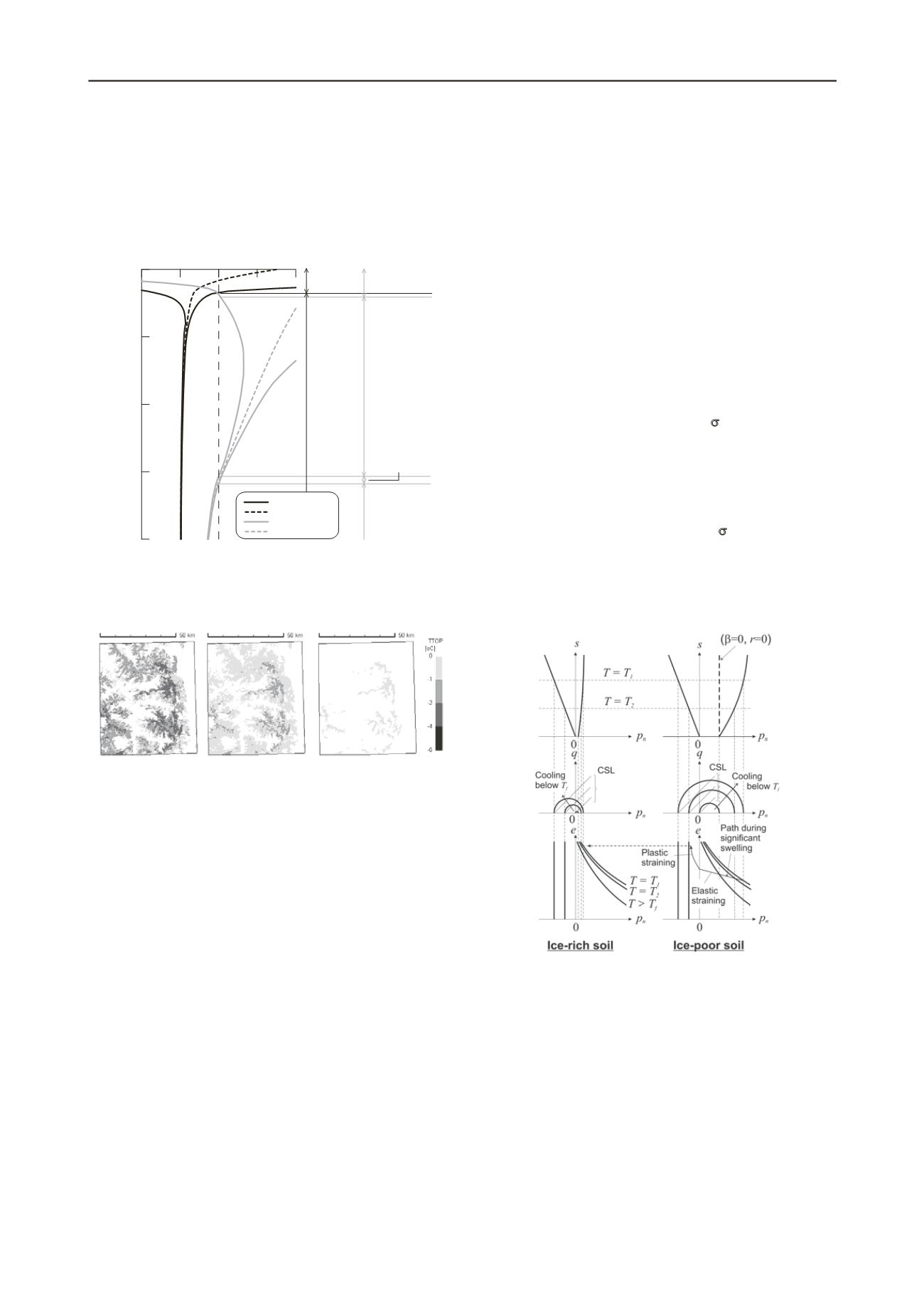
An example of the computational output is given in Figure 4,
showing seasonally transient ground temperature-depth
‘trumpet’ curves for years 2000 and 2050. The climate warming
effects are clear, with the permafrost table lowering and
permafrost warming; effects are more dramatic near the surface
than at depth.
20
15
10
5
0
Depth [m]
-1
-0.5
0
0.5
1
Temperature [
o
C]
Active layer Active layer
Permafrost
Permafrost
Perennially
unfrozen
Seasonally
frozen/unfrozen
2000
2059
2000 Max&Min
2000 Mean
2059 Max&Min
2059 Mean
Figure 4. Computed annual temperature profiles for 2000 and 2059;
Rolling Hills study area at 643mASL, n-factor = 0.6. Stratigraphy
involves 1-m surface layer with porosity 0.4, decreasing to 0.04 at 15m
depth.
(a) 1940
(b) 2000
(c) 2059
Figure 5. Example of computed TTOP (annual mean temperature at
active layer bottom) for a segment of studied area.
While site-specific geothermal computation is sufficient for
small-scale engineering, strategic planning of large scale
transport or pipeline infrastructure requires regional geothermal
predictions for potentially changing permafrost characteristics.
The three level approach generated maps of key parameters.
The first step was to integrate primary data from remotely
sensed Digital Elevation Models (DEMs) and ground
information such as vegetation canopy cover with geological
databases. These datasets are established with the aid of site
reconnaissance and codified so that a best matching 1-D
analysis case could be associated with any given landscape
point. Once this correspondence has been made, thermal
predictions could be retrieved for the given point from the 1-D
analysis output database. Repeating the process and adopting a
tight grid over the whole surface area allows maps to be drawn.
The first task was to check whether the permafrost distributions
predicted between the 1940s and present times matched current
geothermal and permafrost conditions. Checks against the
regional observations showed that the hindcasts were generally
good, adding confidence to forward predictions. Figure 5
presents examples of TTOP maps at three stages of the analysis
in a 60km by 80km study area showing clear warming of the
permafrost being predicted at higher elevations of the Rolling
Hills study area (after Nishimura et al., 2009a).
4 SOIL-STRUCTURE RESPONSE LEVEL PREDICTIONS
The lowest-level analyses aim to predict how soil-structure
systems will respond to changing geothermal regimes. These
interactions involve coupled physical processes, such as frost-
heave in roads and around chilled pipelines, slope instabilities
due to ground thawing and bearing capacity losses in piles and
shallow foundations due to ground warming. Such problems are
most rationally approached by adopting fully coupled THM
analyses. The details of the THM model developed for this
purpose are described by Nishimura et al. (2009b) and its
essence is summarised below.
The broad framework of the proposed model involves the
classical THM elements described by Gens (2007): equilibrium
of forces; coupled mass and heat conservation; the Clausius-
Clapeyron equation of phase equilibrium; permeability and
thermal conductivity functions and a variety of models
describing non-linear freezing and mechanical behaviour. The
state variables include the total stresses,
, the pore liquid water
pressure,
P
l
, and the pore ice pressure,
P
i
. A novel feature of the
proposed model is its mechanical constitutive mode expressing
seamless transitions between frozen and unfrozen states. The
mechanical model is developed from the Barcelona Basic
Model (Alonso et al., 1990) for unsaturated soils, noting a close
analogy between phase interactions in unsaturated soils and
frozen soils. By adopting the ‘net stress’,
-max(
P
l
,
P
i
), and the
‘suction-equivalent’,
max
(0,
P
l
-
P
i
), a Critical-State type elasto-
plastic formulation was made possible while capturing
temperature’s effects via changes in these stress variables, as
illustrated in Figure 6. The Clausius-Clapeyron equation is the
key relationship relating pressure variables to temperature.
Thawing layer
Figure 6. Schematic illustration of yield surface changes according to
temperature changes in the newly developed mechanical model
Examples of the model’s predictions for triaxial compression
are shown in Figure 7. In the top-left diagram, higher strength
develops at lower temperatures, a well-known feature of frozen
soils. The stress-paths followed in accordance with the elasto-
plastic scheme illustrated in Figure 6, are plotted in the right-
hand side diagrams.
Validation of the THM-analysis was performed by
simulating the Calgary field tests reported by Slusarchuk et al.
(1978) on buried chilled pipelines. Pipes of 1.22m diameter
were buried in initially unfrozen silty ground with the invert at
2.0m depth (‘control’ case C) and at 2.9m (the ‘deep burial’
case D). The pipelines were cooled internally from +6.5
o
C to -
8.5
o
C over 50 days, after which the temperature was kept
constant. Figure 8 shows the computed and observed ground


