3392
Proceedings of the 18
th
International Conference on Soil Mechanics and Geotechnical Engineering, Paris 2013
2 HIGH-LEVEL CLIMATIC PREDICTIONS
The study area considered is located in Eastern Siberia. A
regional engineering geology evaluation was made first based
on desk study data, remote sensing information and limited
ground reconnaissance. A set of five stereotypical terrain units
was established. Global climate data were derived for the area
by considering the full ensemble of predictions from the 17
coupled AOGCM models included in the IPCC Fourth
Assessment Report (IPCC, 2007). Their outputs depend on
future greenhouse gas emission emissions using the SRES A2
scenario; a standard, marginally pessimistic projection.
Statistical assessments were made by a team from Department
of Physics at Imperial College to provide multi-model ensemble
mean trends for future, seasonally varying, air temperatures (2
m above ground) and mean snow depth. These were compared
with the locally observed dataset (ERA-40, from the European
Centre for Medium-Range Weather) covering 1958–1998.
Corrections were applied to the entire AOGCM ensemble time-
series based on the differences between modelled and monthly
mean temperatures over the observed period to eliminate model
bias.
The AOGCM ensemble outputs were discretised into 2.5° x
2.5° (latitude and longitude) grid blocks, equivalent to ≈150km
east-west by 280km north-south blocks in the study area.
Ground elevation corrections were applied based on local
topography to produce mean monthly air temperature and snow
depth time-series, combined with models that described local
orographic enhancement of precipitation and solar radiation.
More details are given by Clarke et al. (2008) and Nishimura et
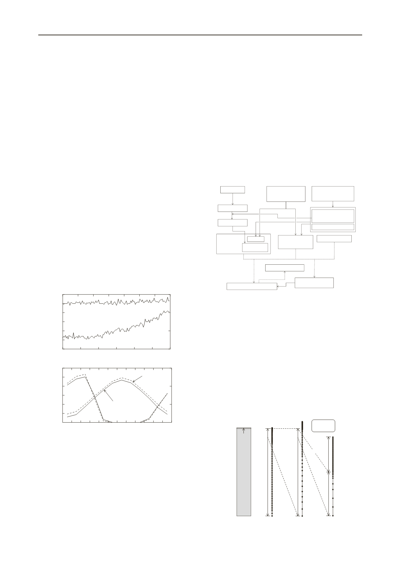
al. (2009a). These processes led to time-series at set elevation
intervals Above Sea Level (ASL) for each terrain type, which
were fed directly into the middle-level analysis. Examples for
the Rolling Hills terrain unit at 643mASL are shown in Figure 1.
1940 1960 1980 2000 2020 2040 2060
Year
-5
-4
-3
-2
-1
0
1
Mean Annual Air Temperature [
o
C]
0
0.2
0.4
0.6
Annual Maximum Snow Cover [m]
Snow cover
Temperature
-30
-20
-10
0
10
20
30
Mean Monthly Air Temperature [
o
C]
0
0.2
0.4
0.6
Snow Cover [m]
Snow cover
Temperature
2050s
Jul: +19.4
o
C
Jan: -20.7
o
C
1940s
Jul: +16.8
o
C
Jan: -23.9
o
C
J F M A M J J A S O N D
Figure 1. Example of predicted time-series for air temperature and snow
cover depth and their monthly averages comparing decadal means
hindcast for the 1940s and projected for the 2050s.
3 MIDDLE-LEVEL GEOTHERMAL PREDICTIONS
Horizontal heat flux is likely to be minor compared to vertical
flow, except in very steeply sloping locations and other limited
localities, so one-dimensional thermal finite element analysis
offered a simple and efficient way of computing time-dependent,
non-linear, ground responses to climatic changes. Air
temperature, snow cover depth and upward background
geothermal flux provided the key boundary conditions.
However, quantitative analysis also required site-specific
geotechnical profiles and topographic information, which is
difficult to assign over wide areas involving variable climate
and geography. The thermal analyses were therefore set into the
broader scheme illustrated in Figure 2 in which a wide range of
potential variables were considered analytically. For example,
local climatic time-series were generated at Rolling Hills
elevations of 343m, 643m, 943m and 1243mASL. Three
different porosity-depth profiles were considered for each to
represent a spread of stratigraphies. Six different ‘n-factors’
were assigned to each to defining a spread of the air-to-ground
heat transfer efficiencies (Lunardini, 1978) that depend on
surface characteristics, such as vegetation type. Finally, two
underlying geothermal flux values were set and a total of 144
analyses run to cover the full range of conditions expected. The
one-dimensional FE analysis outputs were stored and formatted
so that specific information such as temperature at the active
layer base (TTOP), temperature at Zero Annual Amplitude
(TZAA) or permafrost table depth could be recovered swiftly
from the analytical database.
AOGCMs
Local Climate
Local Climate
Surface
boundary
conditions
Geological maps
Field reconnaissance
Satellite images
Remote Sensing
Construction ofDEM
Vegetationcharacteristics
Stratigraphy
(Porosity,watercontent,
freezing function,etc.)
Geothermal flux
-Ensemblemean
-ERA-40scheme
Elevation
-DEM
(Elevation,slopeangle,
slopeaspect, etc.)
-Vegetationcharacteristics
Geothermal Database
1-D FEM
Parametricanalyses
Query
Geothermal map
-n
t
-factor
-Air temperature
-Snowcover
Return
(Conditionsetting)
Figure 2. Structure of middle-level analysis to obtain local geothermal
predictions based on climate predictions and local geography.
The one-dimensional thermal conduction finite element
analysis involved a purpose-written code in which ground
profiles were discretised as shown in Figure 3. Strong non-
linearity in the geomaterials’ temperature-energy relationships
and latent heat effects are captured as well as
porosity/temperature-dependent thermal conductivity. The
conductivity is expressed as a geometric mean of the soil
mineral, liquid water and ice components; the unfrozen water
content below 0
o
C was expressed mathematically. The ground
conditions expected for the 1940-50 decade were hindcasted by
applying the 1940-1950 climate for around 1000 years before
this date to obtain a fully stable initial state. From this point
onwards the computed 1950 to 2050 climate time series were
applied as boundary conditions and the ground response
predicted; see Nishimura et al. (2009a) for details.
100 m
10 m
1 m
119 nodes
59 elements
0.8 m
Snow
elements
Ground
Snow
Figure 3. Discretisation of the ground in 1-D thermal analysis:
Temperature boundary conditions are applied at different snow elements
at different time of a year according to input snow cover depth data.


