1898
Proceedings of the 18t
h
International Conference on Soil Mechanics and Geotechnical Engineering, Paris 2013
EnKF cannot produce satisfactory estimates if its linear
approximation is invalid. This means that its application to
geomaterials is difficult, because the materials display strong
nonlinearity. On the other hand, as the PF does not require
assumptions of linearity or Gaussianity, it is applicable to
general problems. Therefore, the PF has higher potential for
application to geotechnical engineering and can obtain
meaningful outcomes. Brief description of the PF is
summarized below.
The PF approximates probability density functions (PDFs)
via a set of realizations called an ensemble that has weights, and
each realization is referred to as a ‘particle’ or a ‘sample’. For
example, a filtered distribution at time
t
–1,
p
(
x
t
-1
|
y
1:
t
-1
), where
y
1:
t
-1
denotes {
y
1
,
y
2
,…,
y
t
-1
}, is approximated with ensemble {
x
t
-
1|
t
-1
(1)
,
x
t
-1|
t
-1
(2)
,…,
x
t
-1|
t
-1
(
N
)
} and weights {
w
t
-1
(1)
,
w
t
-1
(2)
,…,
w
t
-1
(
N
)
}
by the following equation:
N
i
i
t t
t
i
t
t
t
x x
N
y xp
1
)(
1 1
1
)(
1
1 :1 1
)
(
1 )
(
w
(1)
where
N
is the number of particles and
is the Dirac delta
function.
w
t
-1
(
i
)
is the weight attached to particles
x
t
-1|
t
-1
(
i
)
and
should suffice
w
t
-1
(
i
)
1 and
w
t
-1
(
i
)
=1.
A general approach for filtering is known as sequential
importance sampling (SIS) (Doucet
et al
. 2000). The SIS
algorithm is based on using the importance sampling to estimate
the expectations of functions of the state variables. The
algorithm of SIS is summarized as follows:
1.
Initialization:
Generate an ensemble (set of particles) {
x
0
(1)
,
x
0
(2)
,…,
x
0
(
N
)
}
from the initial distribution
p
(
x
0
).
2.
Prediction:
Each particle
x
t
-1
(
i
)
evolves according to the numerical
dynamic model given by a numerical simulation method
such as FEM.
3.
Filtering:
After obtaining measurement data
y
t
, calculate weight
w
t
(
i
)
,
which expresses the “fitness” of the prior particles to the
observation data, and assign a weight,
w
t
(
i
)
, to each
x
t
-1
(
i
)
.
4.
Weight update:
The set of weighted particles {
x
t
(
i
)
} results in an ensemble
approximation of filtered distribution
p
(
x
t
|
y
1:
t
).
Set
t
=
t
+ 1 and go back to Step 2.
Figure 1 shows the algorithm of the PF based on the SIS.
Prediction
Likelihood
Filtering
x
State space
t
+ 1
←
t
) ,
(
)(
)(
1 1
)(
1
i
t
i
t t
t
i
tt
v xF x
t
y
) ,
(
)1(
)1(
1 1
)1(
1
t
t t
t
tt
v x f
x
1 1
t t
x
1
tt
x
)(
~
i
t
w
Weight
Data
1
tt
x
1
tt
x
Simulation
Weight update
j
(j)
t
j
tt t
i
tt t
i
t
xyp
xyp
1
) (
1
)(
1
)(
)
(
)
(
~
w
w
Figure 1. Algorithm of the PF based on SIS.
3 PARAMETER IDENTIFICATION OF CAM-CLAY
MODEL USING THE PF
This chapter focuses on the soil-water coupled behavior of a
clay foundation under monotonic loading, where the numerical
simulation for hypothetical soil deposit under embankment is
implemented to study the efficiency of the PF as a parameter
identification method.
The soil-water coupled finite element analysis using the
Cam-clay model were used in this example. The finite element
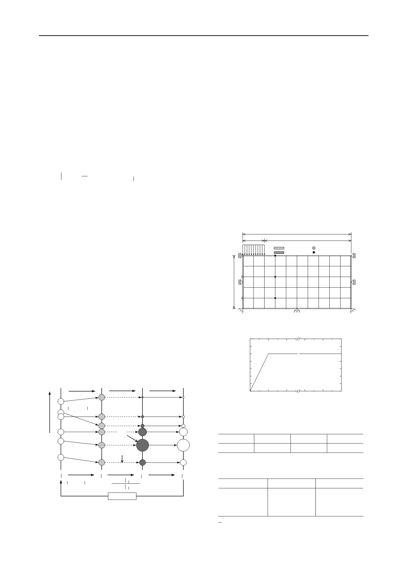
mesh and the loading history are shown in Figures 2 and 3,
respectively. Table 1 lists the parameters of the clay foundation.
The placement of the observation points is also shown in Figure
2; the vertical displacements and the horizontal displacements
are located at S1-S3 and at L1-L3, respectively. Some of the
parameters are chosen to be identified and their values are
called ‘true values’ as listed in Table 2, and we carried out 100
Monte Carlo Simulations using the sets of particles which were
generated with uniform random numbers in the range shown in
Table 2.
Figure 4 shows the time evolution of the identified
parameters (
,
, and
. Identified parameters are computed as
the weighted mean value of the particles computed by
: Permeable
: Impermeable
S1
S2
S3
L1
L2
L3
50.0
100.0
20.0
80.0
( Unit : cm)
: Lateral displacement
: Settlement
Figure 2. Finite element mesh.
0
10
20 111480 111490 111500
0
10
20
30
40
50
60
70
Elapsed time (min)
Applied load (kPa)
Figure 3. Loading history.
Table 1. Cam-clay parameters of the model foundation.
e
0
0.190
0.065
0.992
1.154
Table 2. True values of the parameters to be identified and range
of particle generation.
Parameter
True value
Range
0.239
0.090 ~ 0.290
0.091
0.015 ~ 0.115
1.084
0.854 ~ 1.454
N
i
i
t
i
t
t
1
)( )(
w
(2)


