1903
Technical Committee 206 /
Comité technique 206
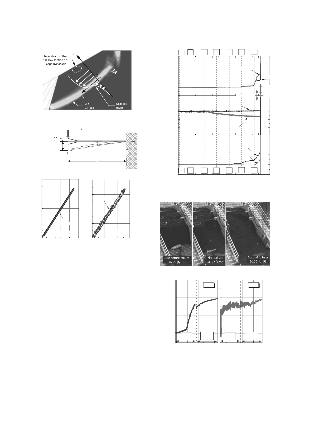
Figure 5. Schematic image of distribution of shear strain at slope failure.
L
Set t l ement
Fi xed end
Load
Out put
I nt erpr et ed shear st rai n
﴾
Negat i ve i n t he di rect i on
﴿
a) Outline of method for calibration of MPS
0.0 0.3 0.6 0.9 1.2
0
200
400
600
800
Out put
r
s
(
)
Interpreted shear strain
(%)
r
s
=653.5
s
Coefficient of
correlation 0.99
0
2
4
6
0
2
4
6
8
Load
F
(N)
Settlement
s
(mm)
F =1.31 s
Coefficient of
correlation 0.99
b) Electrical output
r
s
and interpreted shear strain
c) Load
F
and settlement
s
Figure 6. Stiffness and sensitivity of MPS
A calibration of MPS was carried out to investigate the
relationship between the electrical output from MPS
r
s
(
) and
the interpreted shear strain
(%).
was defined as the ratio of
the settlement
s
to the effective length
L
of MPS as shown in
Equation 1.
100
(%)
L
s
( 1 )
A vertical load
F
was applied to the end of MPS that was
supported by cantilever beam as shown in Figure 6. A clear
linear relationship is obtained between
r
s
and
as well as
between
F
and
s
. Since 653
in
r
s
was output at 1% in
, a
high resolution on the shear strain was confirmed.
5 EXPERIMENTAL ANALYSES ON MOVEMENT IN
SLOPE
5.1
Comparison of reactions by sensors
Figure 7 shows the reactions from three kinds of the monitoring
sensors. Horizontal axis means the actual time at the test. The
first cutting (S1) begun at 13:00 and the final cutting (S7) was
completed at 16:20. The slope collapsed twice at16:27 and
16:36. This meant that 7 minutes remained prior to the first
failure and 16 minutes existed up to the second failures after the
completion of S7 as shown in Photo 2. An increase of values
appeared in each curve as reactions to increase of potential risk
of slope failure.
13:00 13:30 14:00 14:30 15:00 15:30 16:00 16:30 17:00
- 10
0
10
20
30
- 2
- 1
0
1
0.2
0.0
- 0.2
- 0.4
- 0.6
- 0.8
DT P1
S4
S3
S2
Displac ement
d
(mm)
T ime
S1
S6
S5
DTP2
S7
ASG2
A ngle of inclinat ion
a
(deg)
ASG1
16:27
First failure
MPS2
Int erpret ed shear st rain
(%)
MPS4
16:36
Second
failure
S1 S2
S3 S4
S5 S6
S7
Figure 7. Comparison of reaction of sensors in the model test
Photo 2.Process of failures in the model slope
0
5
10
15
0.0
- 0.2
- 0.4
- 0.6
Second
failure
Second
failure
First
failure
ASG1
Int erpret ed shear st rain
(%)
Displacement
d
(mm)
MPS4
First
failure
0
5
10
15
0.0
- 0.4
- 0.8
- 1.2
Angle of inclination
a
(deg)
Displacement
d
(mm)
Figure 8. The relationship between the interpreted shear strain
and the
displacement
d
(in left) and the relationship between the angles of
inclination
a
and
d
(in right).
First small increase can be seen at S3 in
and its value
shows the step increase from S3 to S7. After S7, however,
values of
kept on increasing from 16:20 to 16:27. Both MPS2
and MPS4 installed at the upper side of the slope show the same
increase. Both two curves bent at 16:27 when the first failure
occurred. Moreover, values of
were built up again at 16:36 of
the second failure.


