1544
Proceedings of the 18
th
International Conference on Soil Mechanics and Geotechnical Engineering, Paris 2013
density is the same regardless of the depth; 3) within a layer, the
specific volume and degree of structure is assumed to be
constant, and the overconsolidation ratio is assumed to be
distributed in accordance with the overburden pressure; 4)
Initial stress ratio
η
and degree of anisotropy ζ are both assumed
to be constant as 0.545 for every layer
2.2
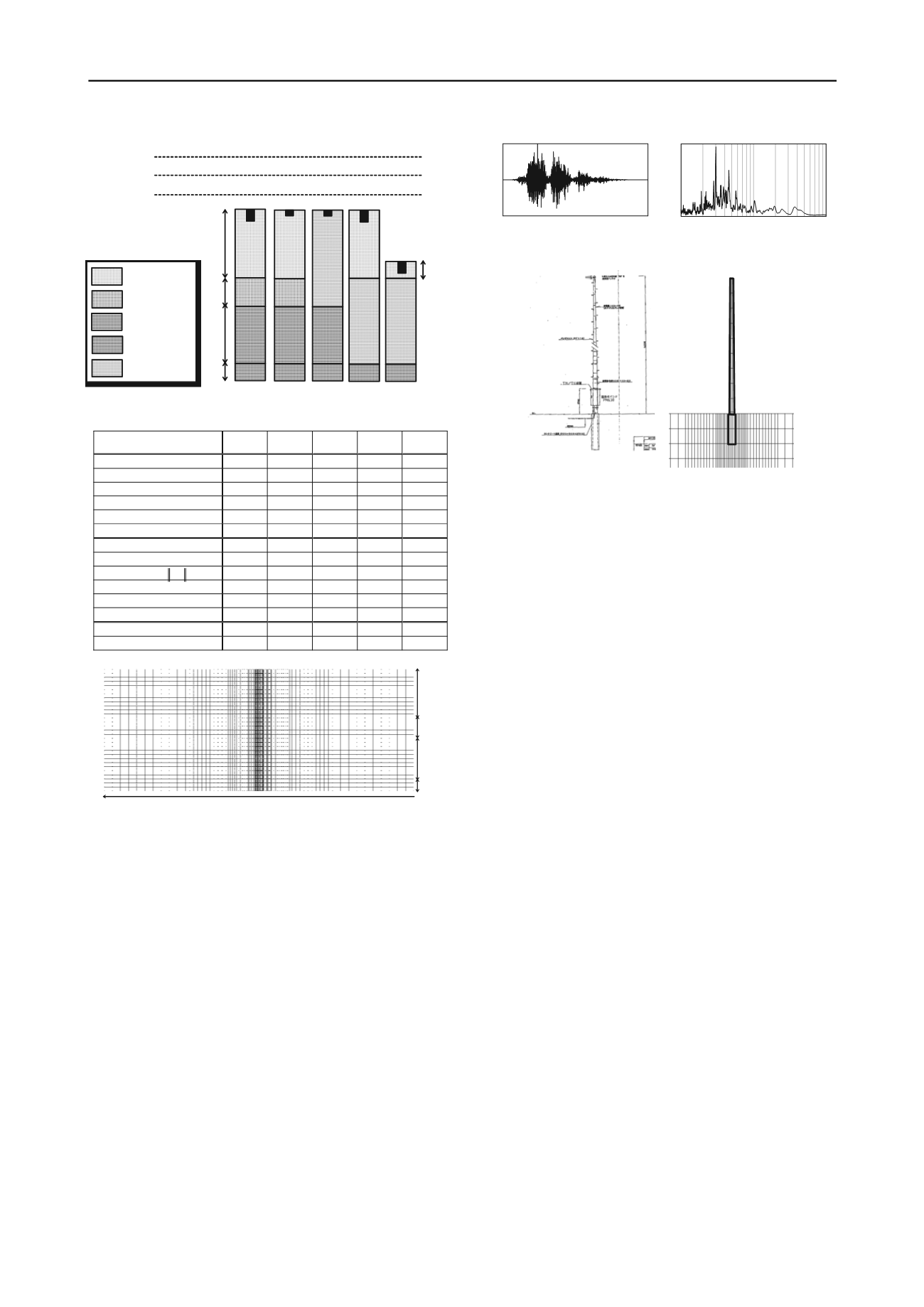
Finite element mesh and input seismic waves
Fig. 2 indicates the finite element mesh. The area analyzed is
of a width of 76.1 m and a depth of 30 m (in Case 5 only, the
depth was 21 m). The hydraulic boundary conditions are set so
that the ground water level coincides with the ground surface
where the water pressure is zero; considering the existence of
impermeable layers with a small coefficient of permeability, the
bottom surface is set as an undrained boundary, together with
the two side surfaces. Also, to provide cyclic boundaries as
constraint conditions, an equal displacement condition is
applied to all components of all nodes at the same height on the
two side surfaces. Fig. 3 shows the input seismic wave adopted
in the analysis. This seismic wave is based on the Tokai,
Tonankai and Nankai triple segment type earthquake as defined
by the Central Disaster Management Council for around the
Nagoya Port area, modified in accordance with the value of the
Vs. A viscous boundary is set on the bottom surface
corresponding to Vs=570 m/sec.
2.3
Modeling the structure
The candidate for analysis is a lightweight, long and slender
steel fabricated column with a bottom diameter 0.3m, column
height 15m, and weight of 2.4kN. The concrete part embedded
in the ground and the column was modeled as a homogeneous
elastic material with uniform weight and stiffness, considering
the actual structure (Fig. 4). The practical column is embedded
to a depth of 2 to 3m as a measure against toppling over in the
earthquake, but in this analysis, a hypothetical dangerous case
with an embedment depth of 1 m is also involved.
3 ANALYSIS RESULT & DISCUSSION
3.1
Influence of the soil properties of the surface layer
In order to understand the seismic behavior of the ground itself
at first, Fig. 5 shows the element behavior (mean effective stress
path and stress-strain curve) during the earthquake in the center
of subsurface reclaimed sand without constructing the column.
It can be seen that the stress state reaches almost
p
’=
q
=0 which
means liquefaction, and large shear strain generates during the
earthquake.
Fig. 6 presents the acceleration response and the Fourier
amplitude spectrum at each layer boundary. In the diluvial sand
layer, responded acceleration amplifies specially in the long-
period wave around 0.3s. On the other hand in reclaimed and
alluvial sand layers, acceleration amplifies during the early
stage of the earthquake, but after the stage of maximum
acceleration, responded acceleration attenuates specially in the
short-period wave which is known as characteristic behavior at
the time that liquefaction takes place.
Fig. 7 shows the shear strain distribution 2min after the
earthquake when the embedment depth is 2 m and 1 m
respectively (enlarged diagram around the column). With the
occurrence of an earthquake, shear strain in the surface sand
layer which liquefies becomes large especially around the
embedment concrete. Compare the figure at the time of 1min
after the occurrence of the earthquake, it turns out that the
domain with larger shear strain reaches deeper as the
embedment depth become longer which means the load
assignment is carried out in the depths. Fig. 8 shows a
comparison of the deformation (horizontal displacements and
vertical settlements) at the tips of the column. In Case2 with the
12m
5m
10m
3m
3m
Case1 Case2 Case3 Case4 Case5
Fs
As
Ds
M
Reclaimed Sand
Alluvial Sand
Diluvial Sand
Mudstone
Embedment depth 2m 1m 1m 2m 2m
Foundation type A A B C D
Ac
Alluvial Clay
As
Fs
Fs
Fs
Ac
Ac Ac
As
Ds
Ds
Ds
M M M M M
Figure 1. Stratigraphic organizations and embedment depth for analyses
Table 1 Material constants for soils
M
Ds
As
Rs
Ac
Elasto-plastic parameters
Critical state index M
0.60
1.10
1.10
1.10
1.60
NCL intercept N
2.10
1.989
1.989
1.989
2.51
Compression index
~
0.17
0.05
0.05
0.05
0.21
Swelling indes
~
0.003
0.0002
0.0002
0.0002
0.02
0
50
100
150
-300
0
300
Time (s)
Fourieramplitude (gal*s)
Poisson’s ratio
0.3
0.3
0.3
0.3
0.3
Evolution parameters
Degradation index of structure
a
0.01
5.0
5.0
5.0
0.6
Ratio of
p
v
D
to
p
s
D
s
c
1.0
1.0
1.0
1.0
0.3
Degradation index of OC
m
10.0
0.12
0.12
0.12
5.0
Rotational hardening index
br
0.001
3.0
3.0
3.0
0.001
Limit of rotational hardening
b
m
1.0
0.9
0.9
0.9
1.0
Soil particle density
s
(g/cm3)
2.707
2.675
2.675
2.675
2.754
Mass permeability index
k
(cm/s)
1.0
×
10
-7
4.0
×
10
-3
4.0
×
10
-3
4.0
×
10
-3
1.0
×
10
-6
3m
10m
5m
12m
76.1m
Figure 2. Finite element mesh and boundary conditions
Acceleration (gal)
10
-1
10
0
10
1
0
300
Period (s)
Figure 3. Input seismic wave and
Figure 4.
Modeling of the steel fabricated column


