1425
Technical Committee 203 /
Comité technique 203
Proceedings of the 18
th
International Conference on Soil Mechanics and Geotechnical Engineering, Paris 2013
sections.
displacements increase for a given k
y
/k
max
ratio, with increasing
PGA
input
.: for PGA
input
=0.1g, the calculated average
displacements plot on the lower bound of the Makdisi and Seed
(1978) curves, for PGA
input
=0.2g they plot between the two
bounds, but still closer to the lower bound curve, for
PGA
input
=0.3g the displacements fall between the upper and
lower bound curves, and finally for PGA
input
=0.4g they plot
closer to the upper bound. A similar pattern can be seen for the
bin M
w
=7.5. This provides an important insight as to how to
interpret these bounds proposed by Makdisi and Seed (1978) for
different shaking intensities, within the same magnitude bin.
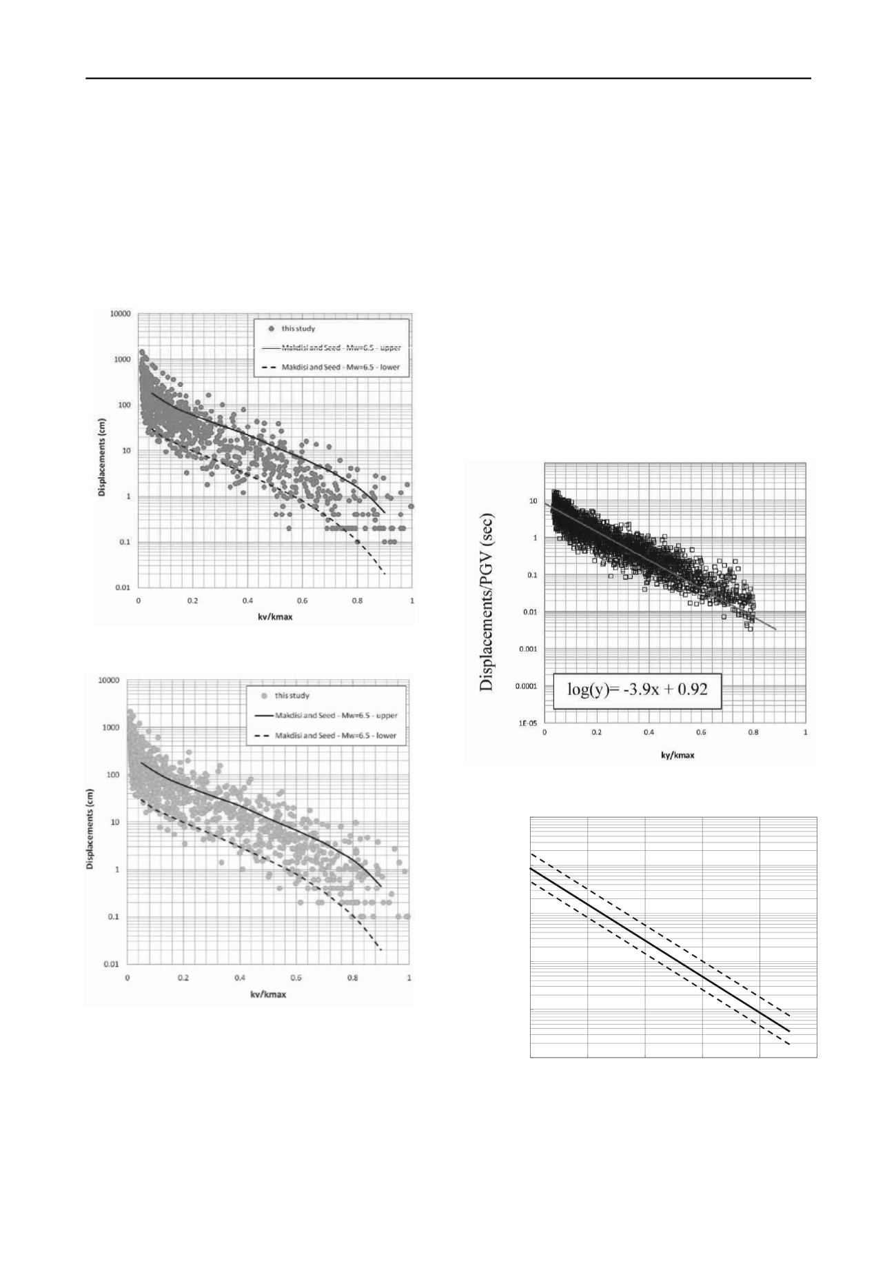
Figure 5.Seismic displacements for motions with M
w
=6.5 to 7.0 and
PGA
input
=0.3g, for Levee A.
Figure 6.Seismic displacements for motions with M
w
=6.5 to 7.0 and
PGA
input
=0.4g, for Levee A.
The scatter, as can be seen from the displacement plots, is
significant and represents the variability of the dynamic
response due to the wide range of ground motions that were
used in the analyses. In an effort to reduce the scatter a group of
parameters that seemed more promising were examined for
normalizing the seismic displacements [i.e., peak ground
acceleration (PGA
input
), peak ground velocity (PGV
input
),
seismic demand (k
max
), mean ground motion period (T
m
),
significant duration (D
5-95
), arias intensity (Ia) and site period
(T
s
)]. Detailed results for all parameters can be found in
Athanasopoulos-Zekkos (2008, 2010).
In summary, it was found that the PGV
input
is the intensity
measure that correlates the best with seismic displacements for
stiff sites (T
s
= 0.45 to 0.58sec) with weak slopes (k
y
=0.05 to
k
y
=0.1). This can be explained since PGV
input
is less sensitive to
high frequencies and is also a good proxy for intensity as well
as duration for short period structures, as is the case with
earthen levees. PGV
input
2
was also examined (Newmark, 1965),
but it did not give a better correlation than PGV
input
. An
additional advantage to PGV is that it can be directly estimated
using the New Generation Attenuation (NGA) relationship
models, for a given earthquake scenario (Boore and Atkinson,
2008, and Campell and
Bozorgnia, 2008). As shown in
Figure 7 the
normalized seismic displacements follow a linear trend in a
semi-logarithmic plot. The standard deviation for all regressions
for the three levee cross sections is on average 0.3 in log units. .
After compiling the regressions for all sliding surfaces and all
intensity levels the lines shown in Figure 8 are recommended
for evaluating seismic displacements for the three levee cross-
Figure 7. Normalized seismic displacement for the deeper sliding
surface on the waterside of Levee A, PGA
input
=0.2g
Figure 8. Recommended normalized seismic displacement lines (16%,
50% and 84% probability of exceedance) (all PGA
input
).
0.001
0.01
0.1
1
10
100
0
0.2
0.4
0.6
0.8
1
Displacements/PGV(sec)
ky/kmax


