1424
Proceedings of the 18
th
International Conference on Soil Mechanics and Geotechnical Engineering, Paris 2013
Proceedings of the 18
th
International Conference on Soil Mechanics and Geotechnical Engineering, Paris 2013
estimates of dynamic response of levees for the three different
levee sites and to also provide insight towards the effect of
ground motion selection to the dynamic response of earthen
levees. The ground motions were selected from the Pacific
Earthquake Engineering Research (PEER, 2007) Center, NGA
strong motion database. Four groups of input ground motions
were used in the analyses, each group scaled to a specified
PGA
input
: 0.1g, 0.2, 0.3g, and 0.4g respectively.
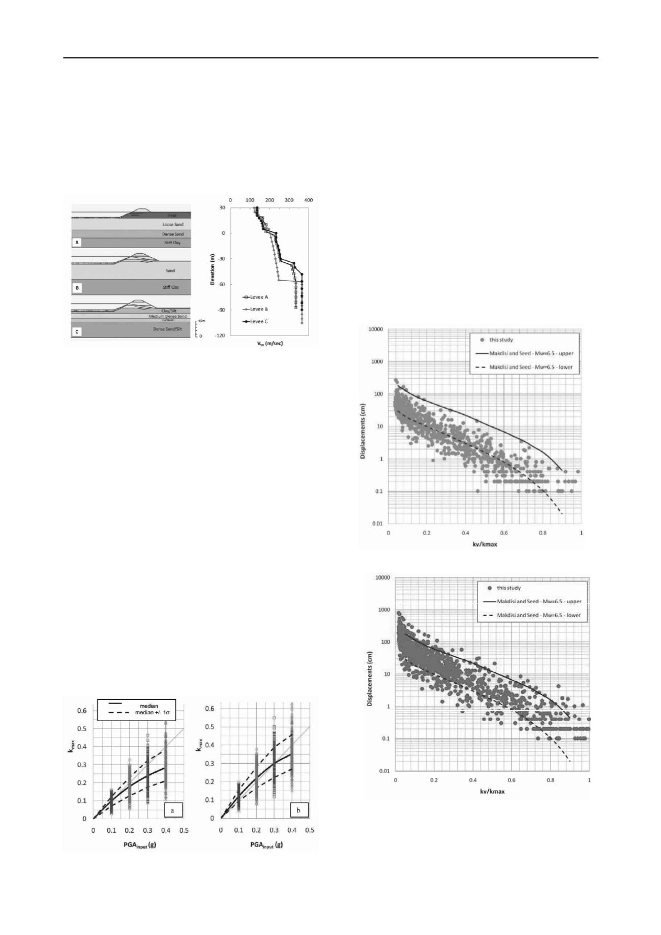
Figure 1.Levee geometry and soil stratigraphy and corresponding shear
wave velocity profile for levee sites A, B and C. Elevation 0m is at the
ground surface on the landside (from Athanasopoulos-Zekkos, 2010).
Four sliding surfaces were pre-selected based on previous
slope stability analyses (URS 2008) for identifying the most
critical sliding surfaces, and the seismically induced deviatoric
displacements were computed using a Newmark-type approach.
In the original Newmark method, the sliding mass is considered
to be a rigid block, however in this study its dynamic response
was also considered. As suggested by Seed and Martin (1966),
the effects of the dynamic response of the sliding mass itself can
be significant in the overall displacements. Therefore, the
concept of the equivalent acceleration time history is used to
account for this effect. The approach followed in these analyses
is a decoupled, equivalent linear model; first the dynamic
response of the potential sliding mass is computed, then the
horizontal equivalent acceleration (HEA) time-history is
calculated and double-integrated, with respect to time, over the
time range that the HEA exceeds a given yield coefficient, k
y
, to
compute displacements. The maximum value of the HEA time-
history (MHEA) is the seismic coefficient, k
max
. and is part of
the output of the QUAD4M analyses. Two pairs of sliding
surfaces were studied as part of this project: one shallow and
one deeper sliding surface on the waterside of the levee and a
similar pair on the landside of the levee.
3 ANALYSIS RESULTS
Due to space limitations only results for Levee A will be
presented. Results for Levees B and C are presented by
Athanasopoulos-Zekkos (2008). The magnitude of the
Figure 2.Results for k
max
(MHEA/g) for the (a) deeper and (b) shallower
sliding surface on the waterside of Levee A.
seismically induced displacements will depend on the seismic
resistance of the earth embankment (k
y
) and the seismic demand
(k
max
). Figure 2 shows the variation of k
max
with PGA
input
, for
Levee A, for two of the sliding surfaces that were studied. The
black solid lines are the medians, and the heavy dashed lines
represent the -/+ one standard deviation ranges.
The seismic displacements are then computed using the
USGS Java-based software (Jibson and Jibson, 2003). The yield
coefficient, ky, is considered to remain constant throughout the
duration of the shaking. As expected, the displacements increase
as the k
y
/k
max
ratio decreases. The displacements also increase,
for any given value of k
y
/k
max
ratio, with increasing PGA
input
.
This can be explained if the following is considered: when
integrating the HEA time-history, even of the MHEA (i.e., k
max
)
and k
y
values are the same, the higher PGA
input
will most likely
have a larger area of HEA, exceeding k
y
, and being integrated
over time to calculate displacements. This effect exists
regardless of the M
w
of the ground motions, and becomes less
pronounced for PGA
input
>0.3g, for the suite of levee cross-
sections studied herein.
Figure 3.Seismic displacements for motions with M
w
=6.5 to 7.0 and
PGA
input
=0.1g, for Levee A.
Figure 4.Seismic displacements for motions with M
w
=6.5 to 7.0 and
PGA
input
=0.2g, for Levee A.
This can be further illustrated by comparing results from
this study with the Makdisi and Seed (1978) displacement
charts, for given M
w
ranges. As Figures 3 through 6 show, for
the moment magnitude bin, M
w
= 6.5, the calculated


