1016
Proceedings of the 18
th
International Conference on Soil Mechanics and Geotechnical Engineering, Paris 2013
Figs. 1(b) to (d) illustrate how this model responds to the
normal contact force
F
n
, the shear contact force
F
s
, and the
contact moment
M
. These contact forces can be computed as:
] ,
min[
nb nn
n
RuK F
(2a)
]
(2b)
,
min[
sb s s
s
RuK F
] ,
min[
rb
m
R K M
(2c)
where min[•] is the operator taking the minimum value;
u
n
,
u
s
and
are the overlap, relative shear displacement, and relative
rotation angle;
K
n
,
K
s
and
K
m
=
K
n
R
/12 are the normal,
tangential and rolling contact stiffness;
R
nb
,
R
sb
, and
R
rb
are the
normal, shear and rolling bond strength.
For simplicity, the inter-particle rolling resistance is ignored
at contacts with broken bonds or without bonds. At these
contacts, the linear contact law applies:
n n
n
uK F
(3a)
] ,
min[
n
s s
s
F uK F
(3b)
where
is the inter-particle friction coefficient;
K’
n
and
K’
s
are
the post-failure normal and tangential contact stiffness.
soil grain
tension
(d)
(c)
(b)
(a)
M
u
s
F
s
F
n
u
n
R
rb
Residual
strength
soil grain hydrate
B
R
nb
1
K
n
K
n
1
R
sb
1
K
s
Residual
moment
1
K
r
compression
R
1
R
2
t
Figure 1. Schematic illustration of (a) MH bonded soil grains and its
response: (b)
F
s
against
u
n
; (c)
F
s
against
u
s
;
and (d)
M
against
Jiang et al. (2012a, 2012b) performed microscopic contact
mechanical test to calibrate the model parameters for a large
number of aluminous rod pairs (with a diameter of 12 mm and a
length of 50 mm) bonded by epoxy and cement. Their study
resulted in a generic criterion for bond failure, forming a
strength envelope in a three-dimensional space with axes being
F
n
,
F
s
, and
M
. The projection of the envelope in
F
s
-
M
plane can
be approximated as an ellipse as the following:
1
2
2
2
2
s
rb
sb
R
M
R
F
(4)
The ellipse varies in size with increasing
F
n
. That is,
R
sb
and
R
rb
are functions of
F
n
. For the case of thick bonds, they can be
computed as follows based on experimental findings if only
normal forces are applied on the bond:
n
t
n
n
c
t
n
s
s
sb
R F F R R F L f
R
)]
/()
[( )
(
m
(5a)
t
n
n
c
t
n
r
r
rb
R F F R R F L f
R
)]
/()
[( )
(
(5b)
where
R
t
and
R
c
are the bond tension and compression strength,
respectively, which can be obtained from tension/compression
test of the cementation materials.
L
s
and
L
r
are the slopes of the
straight line linking
R
t
to the peak shear strength or peak rolling
resistance on the projection plane.
f
s
,
f
r
,
n
and
m
are fitting
parameters to the experimental data. They can be calibrated
from contact mechanical tests as Jiang et al. (2012a, 2012b) did
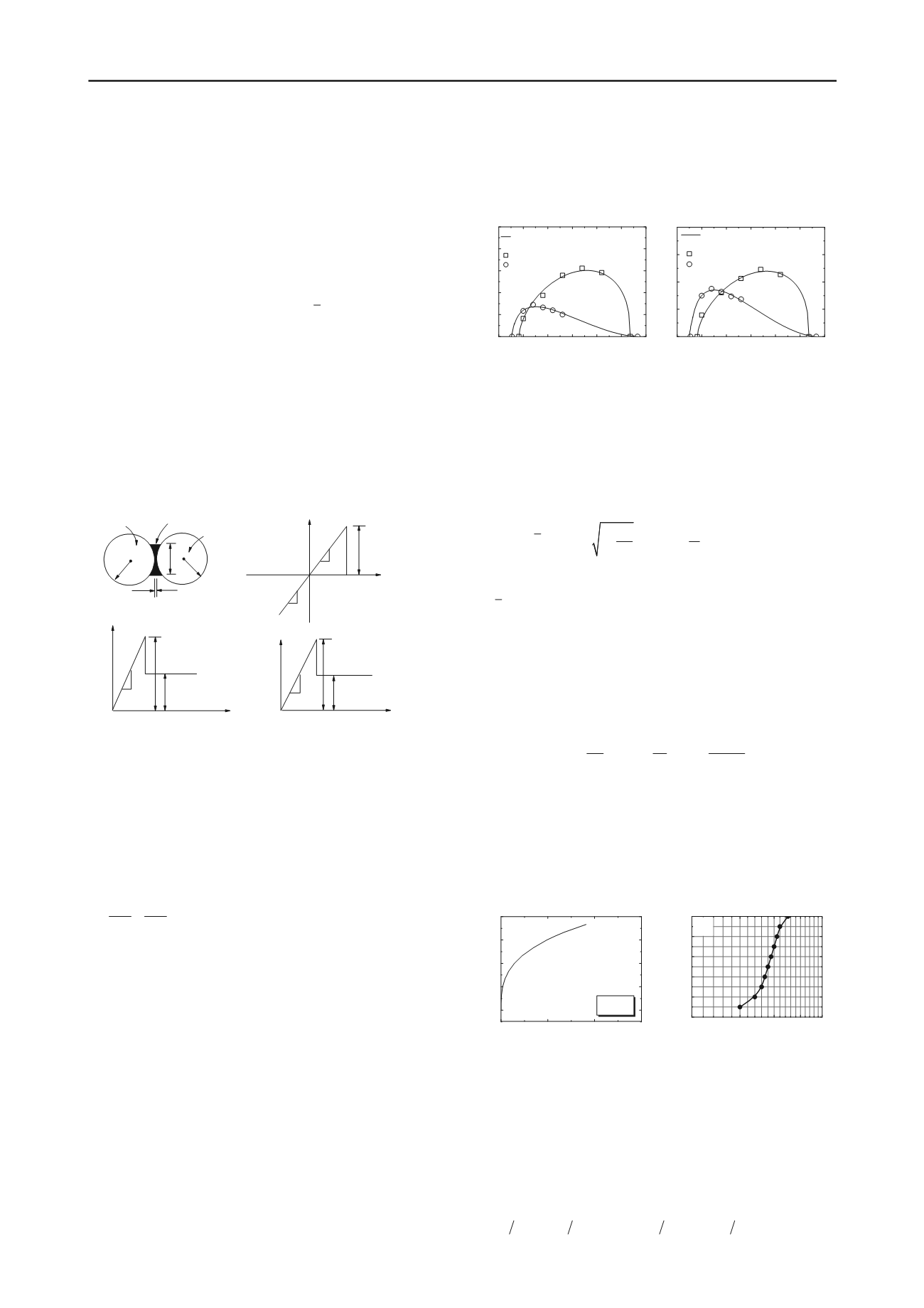
recently. Fig. 2 illustrates their test results with a comparison to
the prediction by Eq. (5).
Since MH remains stable in very extreme conditions, it is
still a challenge to directly measure the strength parameters for
hydrate bonds. Thus, in addition to test data from similar bond
materials, assumptions are necessary for indirectly determining
model parameters for MH bonds. This will be explained later.
-5 0 5 10 15 20 25
0
3
6
9
12
15
Eq. 5a
Test data
(Jiang et al. 2012a,b)
Cement-bonded
Epoxy-bonded
R
rb
(kN
·
m)
F
n
(kN)
(a)
-5 0 5 10 15 20 25
0
2
4
6
8
(b)
Eq. 5b
R
rb
(kN
·
m)
F
n
(kN)
Test data (Jiang et al. 2012 a,b)
Cement-bonded
Epoxy-bonded
Figure 2. Bond strength envelopes derived from laboratory data: (a)
strength envelope for
R
sb
; and (b) strength envelope for
R
rb
2.2
Determing
from
hydrate saturation
The parameter
relates to a given value of hydrate saturation
S
H
, which is defined in a two-dimensional context as the ratio of
the area of voids occupied by MH,
A
H
, to the total void area,
A
V
.
The area of voids occupied by the
i
t
h
MH bond is:
2
2
2
1
2arcsin(
4
bi
i
A R
)
2
(6)
where we assume (1) the radii of the two bonded particles equal
to
i
R
(i.e. neglecting the different curvatures of the particles);
and (2) the bond thickness is negligibly small. The total area
occupied by hydrate bonds,
A
b
, can be found by summation
over all the bonds. Saturation attributed to pore-filling and
bonding hydrates are denoted as
S
Hb
and
S
Hp
, respectively.
S
Hp
,
generally equal to 20-30% (Masui et al. 2005), can be regarded
as the threshold value of hydrate saturation at which MHs start
to bond sand grains. Accordingly,
1
(1 )
(1 )
m
p
b
H
H Hb
Hp
p
Hp
bi
Hp
i
V
e
A
A
S S S
e
S
A S
A
A
A
(7)
where
m
is the total number of bonds;
A
is the total area of a
cross section of the sample;
e
p
is the planar void ratio. Eq. (7)
provides a non-linear relationship which depends on the state of
compaction of the sample (e.g. relative density) which rules the
particle packing and therefore the value of
m
. Fig. 3(a) shows a
sample curve achieved for the case of a dense soil sample (e.g.,
e
p
= 0.21) consisting particles with diameters ranging from 6 to 9
mm forming a gradation curve as shown in Fig. 3(b).
0
10
20
30
0.0
0.3
0.6
0.9
1.2
Parameter
β
nding saturation
S
Bo
4
6
8 10
0
20
40
60
80
100
12
Percentage in mass
smaller than (%)
Particle diameter (mm)
(b)
e
p
=0.21
(a)
H
-
S H0
(%)
Figure 3. (a) Model parameter
at different hydrate saturation for a
dense sample (
e
p
=0.21) with (b) a given gradation curve
2.3
Contact stiffness
Soil grains with the Young’s modulus ranging from 50 to 70
GPa can be regarded as rigid particles relative to MH. Thus, for
MH-bonded grains,
K
n
=
BE
/
t
. The Young’s modulus of MH,
E
,
depends on temperature
T
, confining pressure
p
c
and density
according to the test data (Hyodo et al. 2005). The regression
analysis of these data yields the empirical formula:
0
3
+4950.50
1.98
1821.78
a
c a
w
E p
p p
T T
(8)


