819
Technical Committee 103 /
Comité technique 103
Vreugdenhil at al. (1994), which indicated even a larger value
of approximately
100
ڄ
r
.
The stiffness of the sand layer is apparently independent of
the layer thickness, which becomes evident from the congruent
transition curves when approaching and penetrating the sand
layer. An increase or decrease, respectively, of the stiffness can
be seen, however, for varying relative densities as shown in
Figure 4. A similar result is obtained when varying the clay
strength and the vertical consolidation stress; not shown.
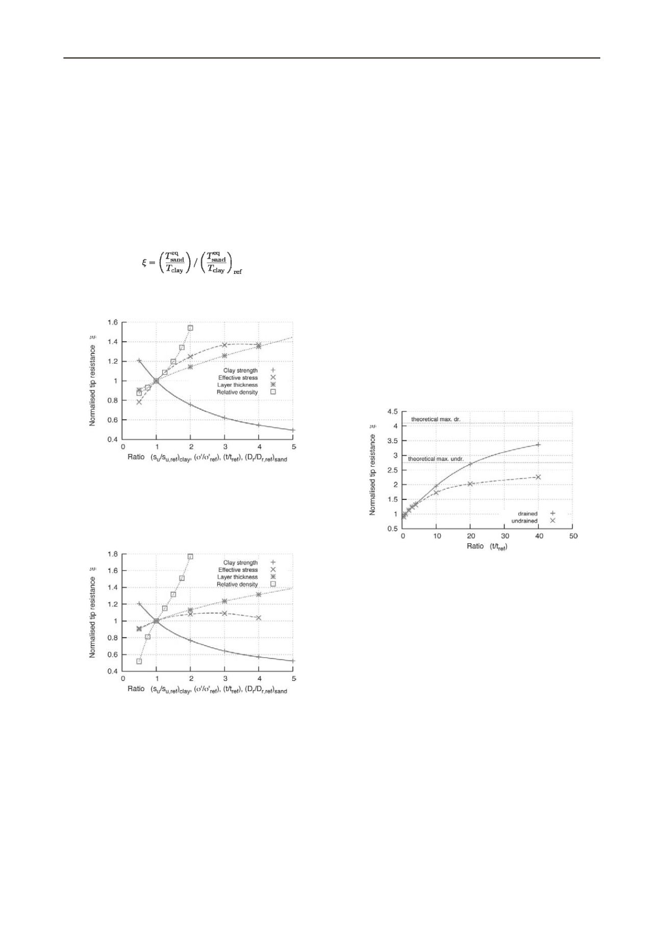
Figure 5 presents the equivalent tip resistance in drained
sand normalised with the equivalent tip resistance of the
reference simulation using the reference parameters listed in
Section 3, viz.
The equivalent strength of the drained sand layer in the
reference model amounts (
T
eq
sand
/T
clay
)
re
f
=3.44
.
Figure 5 Normalised resistance of the drained sand layer depending on
the shear strength of the clay, effective consolidation stress, thickness of
the sand layer and relative density of the sand.
Figure 6 presents the normalised equivalent tip resistance in
undrained sand normalized with the corresponding reference
simulation using the same reference parameters.
Figure 6 Normalised resistance of the undrained sand layer depending
on the shear strength of the clay, effective consolidation stress,
thickness of the sand layer and relative density of the sand.
The curves of the normalized resistances of both drained and
undrained sand are very similar. Almost identical curves are
obtained for varying shear strengths of the clay layer.
The effective consolidation stress has only a small influence
on the resistance in undrained sand, which is plausible since the
relative density governs the undrained strength of sand.
More pronounced is the effect of the relative density being
larger under undrained conditions. The double-bended curve is
somewhat unexpected. However, the resistances at low densities
(
25%
and
37.5%
) are in practice less relevant. Noticeably,
however, is, that the actual values are smaller than expected
based on the diagrams proposed Baldi et al. (1986). But since
the tip resistance in pure sand as measured by Baldi et al. (1986)
can be well reproduced by the FE model using the hypoplastic
formulation (Cudamni and Sturm, 2006), it is believed that the
lower normalised relative resistances at high relative densities
are affected by the layer thickness. The sand is squeezed
horizontally but also vertically into the softer clay which results
in a lower resistance. The squeezing can be well seen in the
deformed mesh when high densities and low undrained shear
strengths for the clay are used. In some cases it lead to distorted
elements introducing numerical difficulties. These simulations
have not been included in the presented diagrams. The vertical
squeezing explains also the higher resistances under undrained
conditions compared to drained conditions. The excess pore
pressure is less than during penetration in pure undrained sand
with similar properties, resulting in higher effective stresses
under the tip and hence higher penetration resistance.
In case of very thin to thin layers, the effect of the thickness
on the penetration resistance is almost independent of the
drainage conditions of the sand. However, when plotting these
curves over a larger range, as shown in Figure 7, it becomes
apparent that the effect is larger under drained conditions. In
addition the theoretical residual maximum normalised resistance
for drained and undrained conditions are plotted in Figure 7.
The curves approaching the theoretical values only
asymptotically, but it is reasonable to assume a value of
approximately
80
ڄ
r
to
100
ڄ
r
as an upper limit at which a further
increase of the thickness has a negligible effect on the
equivalent resistance.
Figure 7 Normalised resistance of the drained and undrained sand layer
depending in the layer thickness.
5 APPLICATION RANGE AND LIMITATIONS
5.1
Application
In order to use the results shown in Figure 5 to Figure 7 for
other design cases than the ones simulated, the different
normalised resistance factors just need to be multiplied. For
example, the normalised resistance of a drained sand layer with
s
u,
clay
=12.5
kPa,
’
v
=200
kPa,
t=2
ڄ
r
and
Dr=100%
is
=1.21·1.25·1.14·1.54=2.66
or
T
eq
sand
=3.44·2.66=9.15·
T
clay
,
respectively, where
T
clay
=N
c
·
·r
2
·s
u,
clay
with
s
u,
clay
=12.5
kPa.
This value agrees well with the result of a corresponding FE
calculation.
The plausibility of this approach becomes apparent from the
following simple example: considering two drained sand layers
with equal density and thickness embedded in normal
consolidated clay but at different depths. The vertical effective
stress and the strength of the normal consolidated clay increase
linearly with depth. The equivalent tip resistance should be then
almost equal in both sand layers, meaning that both effects
should cancel out, given that the sand resistance is stress
independent. This, however, is not the case in the hypoplastic
formulations. Thus, the resistances are only approximately
similar within a range of
±50%
.
In practice, the diagrams are used to estimate the scaling
effects and to provide input for sensitivity studies. Starting point
in most cases will be a CPT profile indicating the presence of a


