233
Technical Committee 101 - Session I /
Comité technique 101 - Session I
Proceedings of the 18
th
International Conference on Soil Mechanics and Geotechnical Engineering, Paris 2013
0
0.5
1
1.5
2
2.5
0
20
40
60
80
100
Settlement/cm
t
/h
r/rw=0.24
r/rw=0.43
r/rw=0.62
r/rw0.8
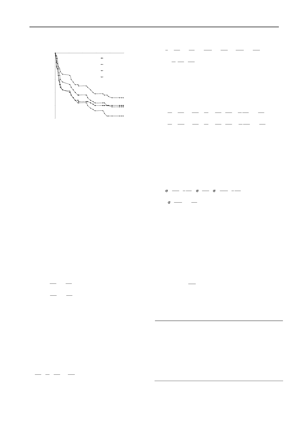
Figure 6. Surface settlements of the soil sample
The surface settlement is shown in Fig. 6. Esrig's theory
about excess pore water pressure indicates that the largest
settlement happens near the anode since the largest excess pore
water pressure is occurred there. However, Fig. 6 shows that the
largest surface settlement occurred in the middle of the two
electrodes with a value of about 2.4 cm. The friction of the test
device and the soil at the anode is the main reason for this
phenomenon.
The test results shows that the soil parameters vary during
the electro-osmotic consolidation processes, and the previous
analytical solution could not adequately predict the soil
behavior due to the complicated coupling effects. The multi-
physics theoretical model was developed by the authors, by
means of coupling soil deformation, pore water flow and
electrical field (Hu et al., 2012).
3 THEORETICAL MODEL
During electro-osmotic consolidation, the pore-water flow,
soil mass deformation, and electricity have a coupling effect on
soil behavior.
3.1
Coupled pore water flow
Pore-water flow is due to the hydraulic and electrical
gradients. The pore water velocity in radial and vertical
directions can be described according to the Darcy's law and
electro-osmotic flow theory (Esrig, 1968),
r
er
z
ez
r
z
H V
v k
k
r
H V
v k
k
r
z
z
(1)
in which
V
and
H
are the electric potential and total head,
respectively;
v
r
and
v
z
are the pore-water flow velocity;
k
r
and
k
z
are the hydraulic conductivity in the radial and the vertical
direction;
k
er
and
k
ez
are the coefficient of electro-osmotic
conductivity
in the radial and the vertical direction,
respectively.
For a saturated soil system with non-compressive pore-water
and soil particles, the pore-water flow induces the volume strain
of soil mass, i.e., consolidation of the soil skeleton. Using the
law of conservation of mass for pore water, the following
equation can be derived,
v
r
r
z
v v v
r r
z
t
(2)
in which
v
is the volume strain of soil mass.
Therefore the governing equation for the pore water
movement in the soil mass can be obtained,
2
2
2
r
er
r
er
z
ez
2
2
2
s
s
1 (
)
(
)
2
2
H V
H V
H
k
k
k
k
k
k
r
r
r
r
r
z
u w
t
r
z
V
z
(3)
3.2
Static equilibrium for soil mass
The elastic constitutive model was used to reflect the
relationship of the stress and the strain of the soil skeleton.
Therefore, the governing equations can be obtained from Biot's
theory and the effective stress principle as,
s
s
s
s
s
3
1
2
3
w
s
s
s
s
s
3
1
2
3
w
(
)
[ (
)]+
(
)
[ (
)]
c
u
w
u w
u
H
c
c
c
r
r
z
z
z
r
r r
r
c
w u
u w
w H
c
c
c
z
z
r
r
z
r
r r
z
s
(4)
in which
c
1
,
c
2
,
c
3
are the constant parameters only related to the
young's modulus and the poisson's ratio;
u
s
and
w
s
are the radial
and the vertical displacements;
γ'
s
denotes the submerged unit
weight.
3.3
Conservation of electrical charge
According to the law of conservation of electrical charge the
governing equation for the electric field can be represented by
the following equation,
2
2
2
er
ez
hr
2
2
2
2
hz
p
2
1
1
(
+ )+
(
+
V V
V
H H
r r r
z
r r r
H V C
z
t
)
(5)
in which
C
p
is the capacitance per unit volume;
er
and
ez
are the electric conductivity in the radial and vertical direction.
hr
and
hz
are the streaming electric conductivity in the radial
and vertical direction, which denotes the current density caused
by a unit hydraulic gradient.
4 NUMERICAL SIMULATION
Based on the equation (3) ~ (5), an axisymmetric electro-
osmotic consolidation model was developed and the size is the
same as the test apparatus. The relationship between the
electrical conductivity and the void ratio is conducted from
laboratory test results as (Wu, 2009),
e
1.016
-0.349 (S/m)
1
e
e
(6)
The soil parameters used in the numerical model are
adopted according to the basic physical properties tests on the
soil sample and are shown in Table. 2 (Wu, 2009).
Table 2. Parameters adopted in the numerical model
Initial water content,
w
/(%)
100
Saturation,
S
/(%)
100
Hydraulic conductivity,
k
r
、
k
z
/(m
s
-1
)
8
10
-10
Electro-osmosis conductivity,
k
er
、
k
ez
/ (m
2
s
-1
V
-1
)
8.5
10
-9
Electrical conductivity,
σ
er
、
σ
ez
/ (1 ohm
-1
m
-1
)
0.38
Young's module,
E
/ (kPa)
2
10
6
Poisson's ratio,
0.3
Fig. 7 shows the comparison of the surface settlement
obtained from the numerical results and the experiment data.
The surface settlement at the position of
r
/
r
e
=0.62, in which
r
e
is


