2693
Technical Committee 212 /
Comité technique 212
coefficients (
α
) and (
β
) was used to define in each layer and the
coefficients were determined from the relationship given below:
i i
i
D
2
2
(1)
where
D
i
= damping ratio corresponding to frequency of
vibration
ω
i
It was assumed that 60 rad/sec and 500 rad/sec were the limit
of predominant frequencies in dynamic testing i.e., all damping
values for different layers were less than the damping values
(
D
1
,
D
2
) considered here in this frequency range. The damping
values were taken from guidelines given by Bowles (1996).
Finally the (
α
) and (
β
) coefficients were calculated by using Eq.
(1).
The model was analysed in three calculation phases. First
gravity analysis was performed only in soil mass in vertical
Z
direction. In the next step, the pile-soil interaction was
introduced as well as static load was applied on the top of the
pile. A steel plate was provided on the pile head to simulate the
exact static load (8 kN and 10 kN) applied on pile. In the third
phase the dynamic FE analysis was performed by applying
sinusoidal vertical load on the pile using a dynamic multiplier
function at wide range of frequencies (5 to 60 Hz). According to
the values of eccentric moments (0.278 Nm, 0.366 Nm, 0.450
Nm and 0.529 Nm) and operating frequency of the motor, the
dynamic load amplitudes were determined.
4 RESULTS AND DISCUSSION
4.1 Validation of finite-element model
To monitor the boundary effect, the model was analysed with
different radius of boundaries. Based on the results, the
boundaries of soil mass around the pile were considered with a
radius of 30 m and height of 45 m to avoid the direct influence
of the boundary conditions. Static load analysis was carried out
and the results obtained from FE analysis were compared with
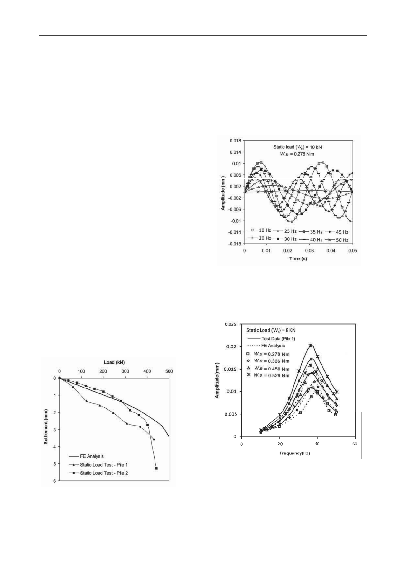
the static load test results. The comparison of static load test
results with the FE analysis is shown in Figure. 3. The predicted
settlement obtained from FE analysis is approximately 1.45 mm
and observed settlement is 1.45 mm and 2.3 mm for pile 1 and
pile 2 respectively at calculated safe load (283 kN).
Figure 3. Comparison of load verses settlement curve obtained from FE
analysis and static load test.
4.2 Comparison between finite-element analysis and dynamic
test results
The time versus amplitude curves were obtained from FE
analysis at different operating frequencies of machine for
different static load and eccentric moments. A typical response
curve is presented in Figure. 4 for static load of 10 kN. From the
time versus amplitude curves, the frequency versus amplitude
curves were obtained and compared with the field vibration test
results.
Figure 4. Time-amplitude response of pile at different frequencies (FE
analysis).
The typical comparison of frequency-amplitude response
obtained from FE analysis and test results are shown in Figure.
5 and Figure 6 for pile 1 and pile 2 respectively.
Figure 5. Comparison of frequency-amplitude curve obtained from FE
analysis and dynamic test results (Pile 1).
It is found from these figures that the predicted resonant
frequency and amplitude are very close to the vertical vibration
test results. The resonant frequencies are decreased with the
increase of eccentric moments under same static load. This
phenomenon indicates the nonlinear behaviour of soil-pile
system obtained from FE analysis which is similar to the field
test results. This nonlinear response of the soil-pile system is
due to the material nonlinearity which is nothing but reduction


