2689
Technical Committee 212 /
Comité technique 212
0
1000
2000
3000
4000
5000
0
1000
2000
3000
4000
5000
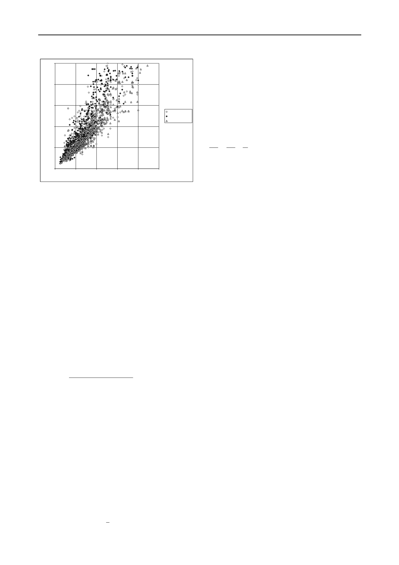
Dynamic Load Tests (KN)
Estimated Bearing Capacity (KN)
Chellis
Uto
Chellis Modificada
Figure 3. Comparison between measured and estimated bearing
capacities using rebound-based dynamic formulas.
5 BAYESIAN UPDATING IN PILE FOUNDATION
SAFETY
Baecher and Rackwitz (1982) define a random variable K =
P
OBS
/P
PRED
as the ratio of observed and predicted resisting
forces, which is assumed to follow a lognormal distribution.
Therefore, R=log
10
(K) is normally distributed (Gauss):
R~N(
,h
-1
), where
and h
-1
are the usual parameters of a
Gaussian distribution;
represents the central tendency and h
-1
the dispersion. In more usual notation, h = 1/
2
, that is,
parameter h, which is sometimes called precision, is the inverse
of the variance. In the context of Bayesian inference, the
parameters of f
R
(r),
and h, are themselves random variables,
so that the (normal) distribution of R is conditional on the
knowledge of those parameters: f
R
(r|
,h). Within this approach:
h
R
R
dh dh f h r f
r f
,
) , ( ) , | (
)(
(1)
The Bayesian updating procedure consists in deriving a
posterior (or updated) distribution f ''(
,h) from the prior
distribution, f '(
,h), and statistics of a sample obtained in the
field. Formally,
-
dh h)d , ( fh) , L(
h) , ( fh) , L(
h) , ( f
'
'
"
(2)
f ''(
,h) is the substituted into equation 1, so as to arrive at an
updated version of f
R
(r).
Variability inherent to geological characteristics of the local
subsoil, driving details and other local and circumstantial
specificities make
2
vary from one site to the next; h is
therefore named intra-site precision. Bilfinger and Hachich
(2006) analyze some aspects of intra-site variability. Baecher
and Rackwitz (1982) treat it as a random variable within the
context of Bayesian inference (see equation 2). Many authors
have treated variance as a known, generally estimated,
deterministic parameter (Kay 1976, Kay 1977, Vrouwenvelder
1992, Zhang 2004). This is the approach adopted here.
Under such conditions of know variance, updating of a
Normal process is significantly simpler and it can be
demonstrated (Martz and Waller 1982) that the posterior
distribution of
, the mean of f
R
(r), is also normal with two
parameters obtained from equations 3 and 4.
rhn mh mh
(3)
hn h h
(4)
The same authors (Martz and Waller 1982) show that, in the
case of known variance, integration of the single nuisance
parameter (
) leads to a predictive distribution of R (equivalent
to equation 1) that is also Normal, with same posterior mean
(equation 5) and a variance that satisfies equation 6.
m m
R
(5)
h h h
R
1 1 1
(6)
The procedure described above can be readily applied to a
situation in which the new information stems from a direct
measurement of the resisting force (P
OBS
), such as a static or
dynamic load test (Hachich and Santos 2006, Hachich, Falconi
and Santos, 2008).
In this paper, however, the idea is to incorporate whatever
information is provided by field control procedures into the
reevaluation of the safety of a pile foundation. The resisting
force on a pile, P
PRED
, is predicted at the design stage by one of
the semi-empirical procedures, which are based on SPT blow
counts from a borehole that is seldom located at the exact point
where the pile is being installed. The only information
pertaining exactly to the location where the pile is installed is
provided by the field control procedures, either set or elastic
rebound, and it would be a waste not to take advantage of this
location-specific information to revise the pile safety prediction.
For this, P
OBS
/P
PRED
can be written as the product of
P
OBS
/P
CLT
and P
CTL
/P
PRED
, where P
CTL
stands for the pile
resistance inferred from the field control records, namely
Janbu’s expression based on set, or Chellis expression based on
rebound. It is straightforward to derive the moments of
P
OBS
/P
PRED
from the moments of P
OBS
/P
CLT
and P
CTL
/P
PRED
. It
is understandable that the variance of P
OBS
/P
PRED
thus obtained
is significantly larger than the variance of the P
OBS
/P
PRED
derived from pile resistances actually measured in pile load
tests. This fact must be accounted for in the Bayesian updating
procedure, since the actual observation is not a pile load test,
but rather an estimate of ultimate load based on a field control
measurement. It can be demonstrated that this is achieved in a
statistically sound manner if the actual number of observations
(n in equations 3 and 4) is replaced by an equivalent number
that is adjusted downwards in proportion to the ratio of those
two variances. In other words, one observation derived from a
set measurement and application of Janbu’s formula (or rebound
and Chellis), is worth less than one observation in the Bayesian
updating procedure.
The moments of P
OBS
/P
CTL
are available from the
proponents of the pile driving formulas and from correlation
studies in the literature. Values relevant to the present
application were presented item 4 above.
Moments of P
CTL
/P
PRED
are the only missing piece of
information for application of the Bayesian updating procedure
just proposed.
Table 3 presents the moments of the random variable
log (P
CTL
/P
D&Q
), estimated from statistical analysis of the
aforementioned database of 189 dynamic pile load tests (Rosa
2000), revised by Bilfinger (2002) to correlate static ultimate
loads to CASE-dynamic ultimate loads. The database includes
precast concrete piles with diameters of 17 to 70cm, lengths up
to 39m, driven by free fall hammers of 13 to 80kN. The first
line of Table 3 refers to the variable log(P
JANBU
/P
D&Q
), while
the second refers to log(P
CHELLIS
/P
D&Q
).


