3034
Proceedings of the 18
th
International Conference on Soil Mechanics and Geotechnical Engineering, Paris 2013
Figure 1. Schematic drawing of an experimental apparatus.
Table 1. Properties of soils.
Silica sand
Andisol
Particle density (g/cm
3
)
2.68
2.40
Mean diameter of particle (cm)
0.085
0.076
Uniformity coefficient (-)
1.80
2.74
Hydraulic conductivity (cm/s)
0.751
0.0341
Porosity (-)
0.42
0.64
Distributor
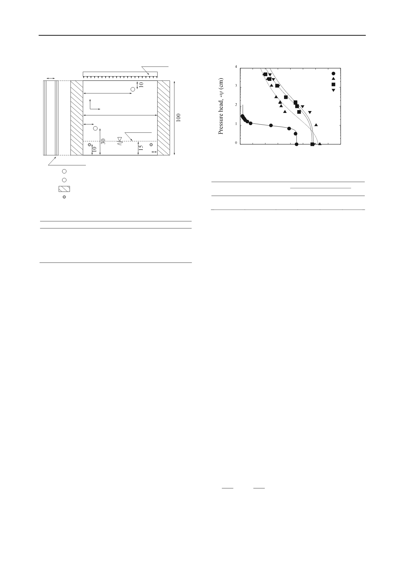
Figure 2. Water characteristic curves for both soils.
Table 2. Experimental cases.
10
10
10
10
10
0 0.1 0.2 0.3 0.4 0.5 0.6 0.7 0.8
Volumetric water content,
(-)
Symbols:
Measured data
Lines:
van Genuchten model
Lab. (Silica sand)
Lab. (Andisol)
Field (20 cm)
Field (50 cm)
2.2 Experimental procedure
Soils were completely washed and saturated before packing to
remove organic chemicals attached to the particle surface, to
avoid entering air and to conduct experiments under the
saturated condition. In the process of creation of flow field,
water flow tank was filled with water and soil material of
interest from bottom to top in 5 cm layers to achieve uniform
packing. In this process, soil was funneled using an extended
funnel. Each layer of interest was compacted prior to filling the
next layer, resulting in 0.42 and 0.64 of the porosity for silica
sand and Andisol, respectively. The porosity of each flow field
was able to be estimated indirectly from measurements of the
particle density and the dry soil bulk density.
After packing, water was applied to the flow tank under a
specific hydraulic gradient controlled by constant head water
reservoirs at the upstream and downstream sides, while
maintaining saturated condition of porous media. A steady
saturated flow field was established when fluctuations in the
observed drainage rate, which was effluent from the constant
head water reservoir, and piezometer readings could become
negligible. After reaching steady state flow conditions, dye
tracer with the volume of 25 cm
3
, which made flow paths
visible, was uniformly injected along the whole thickness of the
flow tank. During the experiment, the profiles of tracer
migration were periodically recorded using a digital camera.
Dye tracer experiments under unsaturated conditions were
conducted in a similar manner. Internal drainage using constant
head reservoirs allowed for one day to create an unsaturated
flow field after the flow tank was filled with water and sand of
concern. After steady state condition was established, water was
applied using a distributor placed 10 cm above the soil surface.
Three rainfall rates of 0.09, 0.21 and 0.63 mm/min, were set
with no rainfall case. Experimental cases are listed in Table 2.
2.3 Image processing and spatial moment approach
Each of the pixels representing an image has a pixel intensity
which describes how bright that pixel is. In order to establish
the relationship between the pixel intensity of a pixel and dye
tracer concentration, a calibration was conducted. Under
identical experimental conditions, a known concentration of dye
tracer was injected into a corresponding porous formation
without a hydraulic gradient. The spread of dye was captured by
the digital camera. The same procedure was repeated using
different concentrations of dye tracer. Consequently, the
concentration of the dye tracer as a function of the pixel
intensity varied over the range of 0 mg/cm
3
to 1.0 mg/cm
3
.
A commonly used measure of dilution is the spatial moments
of aqueous concentrations, which are calculated from snapshots
of tracer plume at given times as follows (Tompson and Gelhar,
1990).
2 ,1 , ,
), ,(
)(
j i
dxdz zxtzxc
tM
j i
ij
(1)
where
x
and
z
are the Cartesian coordinates,
c
is the solute
concentration,
t
is the time,
M
ij
is the spatial moments
associated with the distribution of tracer plume at a certain time,
and
i
and
j
are the spatial order in the
x
and
z
coordinates,
respectively.
The pixel intensity distribution can be converted to a
concentration distribution by the calibration, providing an
analogy between Eq.(1) and Eq.(2).
(2)
2 ,1 , ,
), ,( ) ,(
)(
j i
dxdz zxtzxBzxH
tM
j i
ij
where
H
(
x,z
) is the area per unit pixel and
B
(
x,z,t
) is the
intensity at a corresponding pixel. The centroid of plume
concentration distribution is calculated as the normalized first
order spatial moment by the following equation.
00
01
00
10
,
M
M z
M
M x
c
c
(3)
where
x
c
and
z
c
are the centroid locations of plume
concentration distribution in the
x
and
z
coordinates,
respectively. The second order spatial moments are also
computed as follows.
Rainfall intensity (mm/min)
Soil type
S
0
0.
0.21
0.63
S
S
S-
S-
-
aturated
09
Silica sand
-S
-1
2
3
Andisol
A-S
A-1
A-2
A-3
A-4
Injection port in saturated flow experiments
Constant head water reservoir
100
10
65
S
U
S
U
Water table
Injection port in unsaturated flow experiments
Unit: cm
3
Glass plate
x
z
5
Water pressure measurement port


