2987
Technical Committee 214 /
Comité technique 214
Beratungsgesellschaft mbH. This module is based on a Finite
Difference formulation for simulating borehole heat exchanger
developed by Mottaghy and Dijkshoorn (2012) and has been
modified for the simulation of artificial ground freezing
applications.
Adapted from the Kelvin line source theory the freeze pipes
are modeled as line sources and the horizontal heat transfer is
determined, using the concept of thermal resistances
(Hellström 1991). To realize the coupling of the module
“freezrefcap” with SHEMAT the soil temperature calculated in
SHEMAT T
Soil
is passed to the new module. In turn, a cooling
generation returns to SHEMAT (see Figure 3).
s
Q
„freezrefcap“ „SHEMAT“
T
soil
s
Q
Figure 3. Coupling of “freezrefcap” module and SHEMAT.
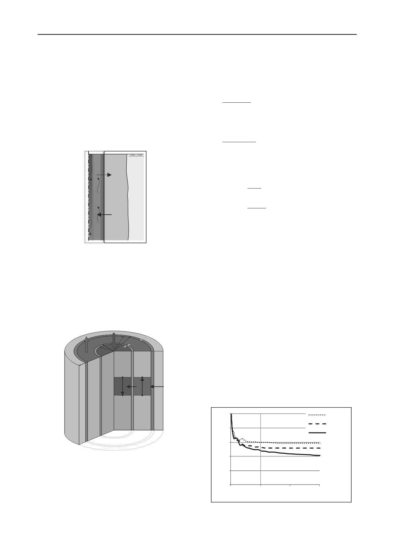
The numerical model includes the afore-mentioned heat
transfer conditions for the calculation of the thermal resistances.
For the numerical model the inner freeze pipe and the annular
space are divided into grid cells that are connected via thermal
resistances (see Figure 4). Assuming a steady state solution the
temperature of all grid cells is calculated considering the heat
balance equation in every time step. Due to the high flow rate
inside the freeze pipes and the comparatively short freeze pipe
length this simplified steady state solution is a good
approximation.
T
in
T
out
r
in
R
inner
r
out
R
outer
r
in‘
r
out‘
r
b
T (i)
d
T (i+1)
d
T (i)
u
T (i+1)
u
s
Q
u
Q
e
Q
d
Q
Figure 4. Calculation basis of module “freezrefcap” according to
Mottaghy and Dijkshoorn (2012).
The module “freezrefcap” offers the opportunity to activate
and deactivate freeze pipes, which provides the basis for the
simulation of different modes during the operating phase. The
distinction between “flow” and “no flow” case requires different
calculations of thermal resistances and the temperature
distribution inside the freeze pipe. In this paper only the “flow”
case is described.
For the determination of the heat flow
s
Q
between the soil
and the outer pipe and between the inner and the outer pipe
the temperatures calculated in the previous time step (t-1) are
used (see Eq. 12 and Eq. 13). The thermal resistances R
inner
and
R
outer
are also calculated considering the results of the previous
time step. Because of the flowing refrigerant the different grid
layers i need to be taken into account.
e
Q
outer
u
soil
s
R
i Ti T
Q
t
1
(12)
For the determination of the heat flow between the outer and
the inner pipe adjacent temperatures in the downstream and in
the upstream are used (see Eq. 13).
inner
d
u
e
R
i T i T
Q
1
t
t
1
1
(13)
The temperature in the downstream T
d
t
(i+1) of the actual
time step t is determined based on the downstream temperature
T
d
(t-1)
(i) of the overlying grid cell i for the previous time step
(t-1) because of the flowing refrigerant.
FF
e
t
d
t
d
cq
Q
i T iT
1
1
(14)
FF
s e
t
u
t
u
cq
QQ
i T iT
1
1
(15)
c
F
indicates the volumetric heat capacity of the refrigerant
and q
F
the flow rate.
Besides the flow rate the inlet temperature or the
refrigeration capacity can be choosen as input parameters.
Furthermore the simulation of different refrigerants requires just
a simple implementation of the temperature dependent fluid
parameters.
3 NUMERICAL SIMULATION
Former numerical simulations at the Chair of Geotechnical
engineering showed that groundwater flow has an important
influence on the freezing process. The results outlined that the
freezing time increases disproportionately and the frost body
development decreases with an increasing flow velocity.
To further investigate the influence of groundwater flow on
the refrigeration capacity a numerical simulation of a simplified
model with only one freeze pipe has been carried out using the
module “freezrefcap”. Because of a missing module validation
against measured data from laboratory model tests only the
qualitative influence of groundwater flow is outlined. For this
example a freeze pipe with an outer diameter of 10 cm, an inner
diameter of 5 cm and a length of 9.5 m has been chosen. The
inner pipe was assumed to consist of polyethylene and the outer
pipe of steel. As refrigerant a 29 % CaCl
2
brine has been
chosen. The results of the numerical simulation are displayed in
Figure 5.
0
1
2
3
4
5
0
100
200
300
Refrigeration capacity P [kW]
Time [h]
v = 2.0 m/d
v = 1.0 m/d
v = 0
Figure 5. Influence of groundwater flow on refrigeration capacity of one
freeze pipe.
It is obvious that an increase in flow velocity causes not only
a reduced frost body development but also an increased


