2935
Technical Committee 214 /
Comité technique 214
4.1
Force vertical and depth penetration of pipe model tests
Figure 3 shows some typical experimental results and a
comparison with those calculated from equations (4), (6) and
(7).
Results presented in Figure 3(a) correspond to the curves of
type
s
u
-
z
/
r
0
(solution of equation 4) which represent undrained
shear strength for each depth of the penetration. The results of
Figure 3a the equation (5) could be used to obtain an average
value of the
s
u
throughout the depth analyzed.
The second type of curves, Figures 3(b) and 3(c),
corresponds to the vertical force
F
v
normalized respect to the
diameter of the pipe and the undrained shear strength (
F
v
/2
r
0
s
u
)
versus the penetration normalized respect to the radius or
diameter. The use of these curves represents the solution of the
equations (6) and (7).
In the case of Figures 3(a) and 3(b) the calculated values
correspond to depths of
z/
2
r
0
0.5, since the theoretical solution
is used for normalized force (Murff et al. 1989, equation 1),
0
2
4
0
0.5
s
u
, kPa
z/r
0
1
Test 10-150-5
= 0
= 1
(a)
0
2
4
6
0
1
2
0 u
z/r
Fv/2r s
= 1
s
u
= 2.7 kPa
= 0
s
u
= 3.4 kPa
est - 50-5
Murff et al. solution
0
,
2
4
1
s
u
, kPa
0
0.5
z/r
0
Test 10-150-5
= 0
= 1
(a)
0
2
4
6
0
1
Fv/2r
0
s
u
= 1
s
u
= 2.7 kPa
= 0
s
u
= 3.4 kPa
Test 10-150-5
Murff et al. solution
2
z/r
0
(b)
0
5
10
15
20
0
0.5
F
v
/2r
0
, kN
z/2r
0
1
Power function solution
s
u
= 3.3 kPa
a = 5.44
b = 0.31
Test 10-150-5
(c)
Figure 3. Estimating of undrained shear strength using a vertical
penetration of a cylinder (Test No. 5). Solution using the equation (4) in
(a). Calculated values of
s
u
considering the solution Murff et al. for
=0
and
=1 (equation 4) in (b). Value of
s
u
by fitting set of experimental
data with a power function solution (equation 7) in (c).
valid for a penetration less than or equal to the radius of the
pipe. Values of the undrained strength calculated considering
two types of surface, while the surface of the laboratory model
was the same during the tests, and that can be interpreted as the
minimum and maximum values.
For the results in Figure 3(c) the adjustment takes into
account the values of z/2
r
0
≥0.5, which represents an advantage
over the equations (4) and (6), and the solution corresponds to a
unique value of
s
u
, also at the same time,
a
and
b
values were
calculated.
4.2
Calculated undrained shear strength
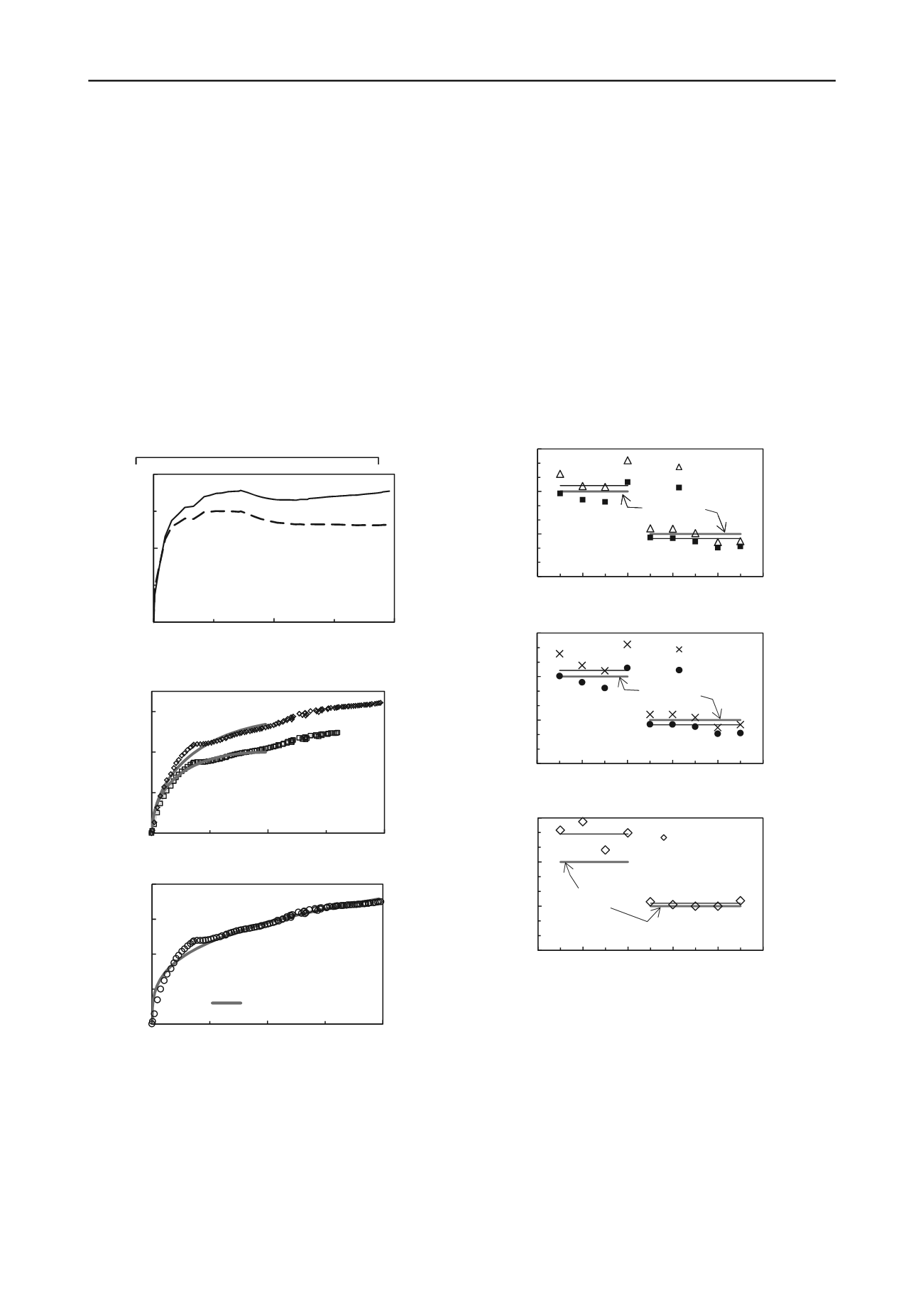
Results of undrained shear strength of all tests are summarized
in Figure 4. Figure 4(a) represents the mean value of the
s
u
calculated with equation (5) for the typical results included in
Figure 3(a). Interpretation of the results takes into account the
variation of pipe surface. It can be noticed immediately the
difference in the results for soils with different undrained shear
strength.
Results are concentrated around the soil resistance obtained
with miniature vane shear test. In case of analysis with
=0 the
estimated values
s
u
are higher than corresponding to a rough
0
3
6
9
0
2
4
6
8
1
Shear strength s
u
, kPa
Test No.
0
su alfa = 0
su alfa = 1
Soil 1
Soil 2
s
u
,
= 0
Vane test
s
u
,
= 0
s
u
,
= 1
(a)
0
3
6
9
0
2
4
6
8
1
Shear strength s
u
, kPa
Test No.
0
su* alfa = 0
su* alfa = 1
Soil 1
Soil 2
s
u
,
s
u
,
= 1
Vane test
(b)
0
3
6
9
0
2
4
6
8
1
Shear strength s
u
, kPa
Test No.
0
su regresion de tipo
potencia
Soil 1
Soil 2
s
u
, Power
function
solution
Vane test
(c)
Figure 4. Undrained shear strength obtained from the equation (5) for a
penetration depth of
z/2r
0
0.5 (a). Values of
s
u
calculated from the
equation (6) and the solution Murff et al. (equation 1) for
=0,
=1 and
z
/2
r
0
0.5 (b). Values of
s
u
calculated from the equation (7) whereas the
total depth of penetration of the pipe model (c).
surface (
=1). Horizontal lines included in the Figure 4(a)
represent the average value of considering all the values of each
soil and roughness. The experimental pipe models used had a
surface intermediate, therefore it is expected that the
corresponding
s
u
value is between two limits.
Figure 4(b) shows the results for the case of the estimated
value from the equation (6). Their values are grouped for each
soil and the tendency of behavior is similar to the results of
Figure 4(a), the difference is clearly distinct between the two


