 
          2943
        
        
          Technical Committee 214 /


            Comité technique 214


          The mud was initially sieved through a 2.36 mm sieve to
        
        
          eliminate all the broken shells and debris and then mixed with
        
        
          sea water at a water content of 270 % in a slurry form. Sea
        
        
          water obtained from Townsville (in Queensland) was used to
        
        
          mix the slurry (Salt concentration 370 N/m
        
        
          3
        
        
          ). The dredged mud
        
        
          slurry was placed in a cylindrical tube of 100 mm diameter and
        
        
          800 mm height and allowed to undergo sedimentation. When
        
        
          the dredged mud column accomplished most of its self weight
        
        
          consolidation settlement, it was sequentially loaded with small
        
        
          weights in the range of 500 to 3000 g. The soil column was
        
        
          allowed to consolidate under each vertical stress increment for
        
        
          two days before the next weight was added. Pore water
        
        
          dissipation was allowed through the porous caps placed at the
        
        
          top and bottom of the dredged mud column. The soil column
        
        
          was loaded up to a maximum vertical stress of 21 kPa over a
        
        
          duration of 8 weeks. The final thickness of the column at the
        
        
          completion of consolidation was around 300 mm.
        
        
          From the final sediment, specimens were extruded for the
        
        
          oedometer tests. Six oedometer specimens of 76 mm diameter,
        
        
          20 mm height, were extruded at three different depth levels as
        
        
          shown in Fig. 2. Three specimens were subjected to standard
        
        
          vertical consolidation tests (denoted by ‘V’) and three were
        
        
          tested to radial consolidation tests (denoted by ‘R’). The
        
        
          procedure for the radial consolidation tests is explained below
        
        
          briefly.
        
        
          Figure 2: Specimen locations for oedometer tests
        
        
          Specimens R1, R2 and R3 were tested for radial
        
        
          consolidation with an outer peripheral drain. The material used
        
        
          for outer peripheral drain was 1.58 mm in thickness. The strip
        
        
          drain was aligned along the inner periphery of the oedometer
        
        
          ring. A special cutting ring of diameter of 72.84 mm was used
        
        
          to cut specimens. The cutting ring had a circular flange at its
        
        
          bottom. A groove was carved along the inner periphery of the
        
        
          flange, which had a thickness equal to the thickness of the
        
        
          bottom edge of oedometer ring plus peripheral drain. The
        
        
          oedometer ring was placed tightly in the groove, to make it
        
        
          align properly with the cutting ring (Fig. 3). The specimen in
        
        
          the cutting ring was then carefully transferred to the oedometer
        
        
          ring using a top cap, without causing any disturbance. The
        
        
          porous bottom and top caps used for standard vertical
        
        
          consolidation tests were replaced with two impermeable caps,
        
        
          for radial consolidation tests.
        
        
          All the specimens were loaded in the oedometer apparatus
        
        
          approximately between a vertical stress range of 9 kPa to 440
        
        
          kPa (9 kPa, 17 kPa, 30 kPa, 59 kPa, 118 kPa and 220 kPa and
        
        
          440 kPa). A load increment ratio of around 1.0 was adopted
        
        
          throughout the loading stage. From the settlement – time data of
        
        
          the specimens under each load increment, the vertical and radial
        
        
          coefficients of consolidation


            c


            v


          and


            c


            h


          were estimated. Taylor’s
        
        
          square root of time method was used for estimating


            c


            v


          .


            c


            h


          was
        
        
          obtained from the curve fitting procedure given in McKinlay
        
        
          (1961) for radial consolidation with a peripheral drain.
        
        
          Figure 3: Specimen preparation for radial consolidation test


            3.1 Results and discussion


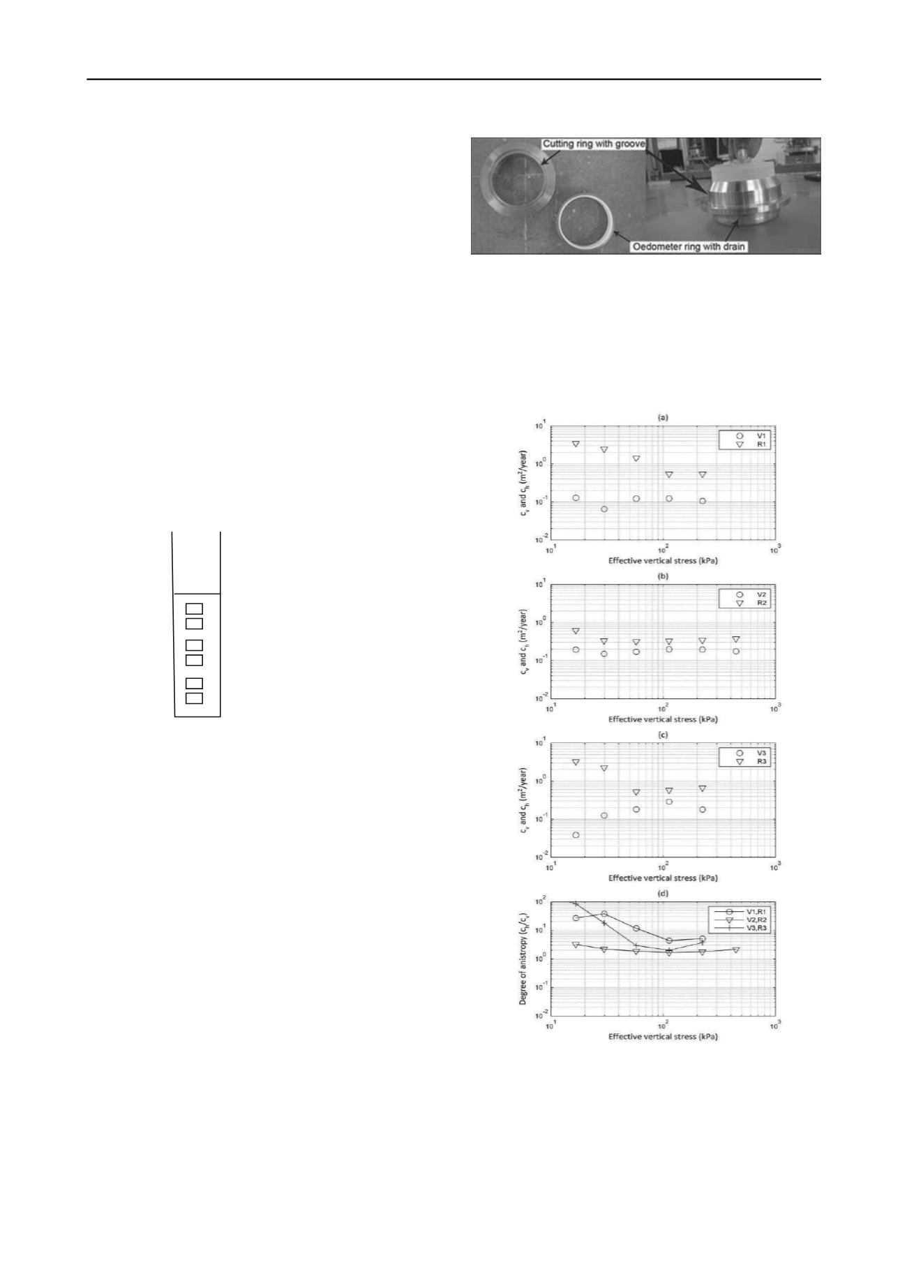
          Figs. 4(a), (b) and (c) show the comparison of


            c


            v


          and


            c


            h


          for pairs
        
        
          V1-R1, V2-R2 and V3-R3 respectively at different effective
        
        
          vertical stresses


            ’


            v


          . The degree of anisotropy, given by (


            c


            h


            /c


            v


          ) is
        
        
          plotted against


            ’


            v


          in Fig. 4(d) for the three pairs of specimens.
        
        
          R3 
        
        
          Notations  
        
        
          V3 
        
        
          R2
        
        
          ‘V’‐ Vertical consolidation 
        
        
          V2 
        
        
          ‘R’‐ Radial consolidation   
        
        
          R1
        
        
          V1 
        
        
          Figure 4: Comparison of


            c


            v


          and


            c


            h


          for specimens (a) V1, R1 (b) V2,
        
        
          R2 (c) V3, R3 (d) Degree of anisotropy
        
        
          As clearly observed, the horizontal coefficient of
        
        
          consolidation is higher than that in the vertical direction at all
        
        
          three depths. The ratio


            c


            h


            /c


            v


          generally decreases with the
        
        
          increase in


            ’


            v


          . At low


            ’


            v


          (


            ’


            v


          < 20 kPa), the ratio


            c


            h


            /c


            v


          varies
        
        
          from 2 to as much as 100. The average degree of anisotropy in
        
        
          permeability (


            k


            h


            /k


            v


          ) for the various stress levels is given in
        
        
          Table 1. The ratio


            k


            h


            /k


            v


          lies between 1 to 4. The horizontal