2934
Proceedings of the 18
th
International Conference on Soil Mechanics and Geotechnical Engineering, Paris 2013
The equation (1) can be represented by an expression of type
power, in function of depth penetration
z
, the radius
r
0
,
coefficient
a
and exponent
b
, as follows:
0
0
2
2
b
v
F
z a
r c
r
(2)
From the above equations, it follows that it is possible to
obtain the resistance undrained shear if the vertical force
F
v
required to penetrate the pipe is known. Considering equation
(1) as the theoretical solution, experimental values and
resistance undrained shear as the unknown value, namely:
0
0
theoretical
experimental
2
2
v
v
u
F
F
r c
r s
(3)
The
s
u
value for each depth of the cylinder penetration is
represented by the equation (4). The undrained shear strength
average for the entire depth
z
is represented by equation (5),
where
N=
total values of cylinder penetration during the
laboratory test.
0 experimental
0 theoretical
2
2
v
u i
v
F
r
s
F
r c
(4)
1
N
u i
u
s
s
N
(5)
Another alternative to obtain
s
u
for the entire depth (
z
) of the
cylinder penetration is solving the equation (3), applying
numerical methods, for instance the least squares method.
In this case, the adjustment evaluation is minimizing the sum
of squared residuals (
E
), which corresponds to the squared
distance of the experimental values and the theoretical curve
based on their, as shown in equation (6).
2
0
0
1
2
2
N
v
v
u i
i
i
F
F
E
r s
r c
(6)
where:
corresponds to the values obtained
experimentally and
s
u
is an unknown;
is the vertical
collapse load normalized by the pipe diameter and the soil shear
strength for different values of
(Murff et al. 1989).
0
/ 2
v
u
F r s
0
/ 2
v
F r c
Substituting equation (2) into (6) it is possible to obtain
E
(equation 7) with three unknowns values: the undrained shear
strength
s
u
, coefficient
a,
and the exponent
b
.
2
0
0
1
2
2
b
N
v
v
u
i
i
i
F
F
E
s a
r
r
(7)
Solution of equation (7) represents the value of
s
u
for the
entire depth (
z
), where the values
a
and
b
allow to fit the
experimental data to approximate the theoretical solution
(equation 1).
Using the expressions (4), (6) and (7) it is possible to obtain
s
u
. Calculated values of
s
u
by these equations were compared
with experimental values as shown in next sections.
3 CYLINDER MODELS AND SETUP
3.1
Cylinder models and setup
Two cylinder models with different geometrical and material
characteristics were used: a steel pipe model with a diameter of
100 mm and a length of 335 mm, the second pipe model in PVC
with 200 mm diameter and 900 mm length.
Tests were performed in the tank
VisuCuve
of Laboratoire
3S-R in Grenoble. Its internal dimensions are 2m-length, 1m-
width and 1m-depth. For the experimental tests it was filled
only 0.4 m-depth with the soft soil.
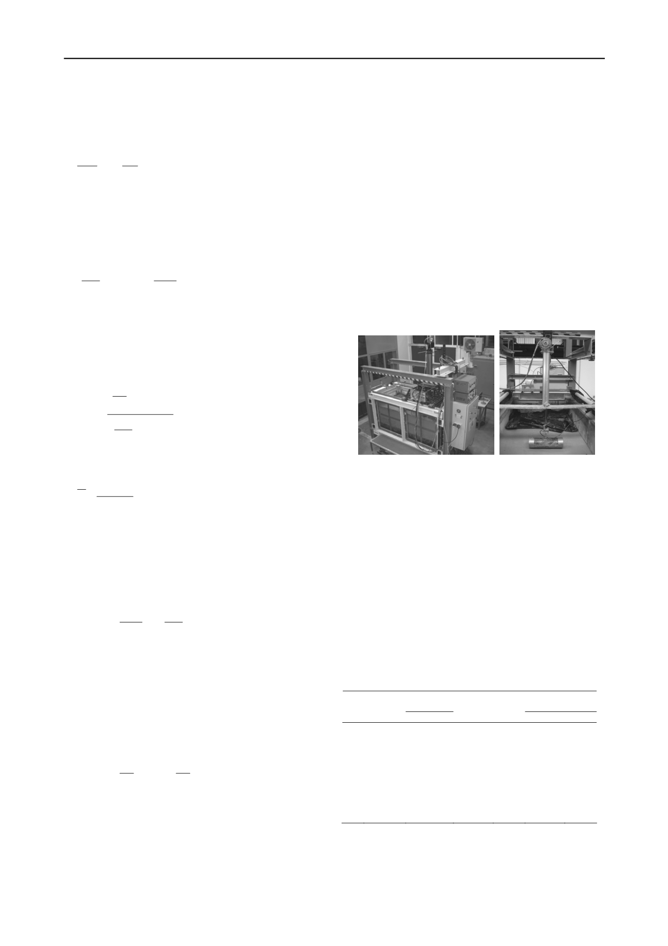
The vertical force
F
v
was applied on the cylinders using an
electromechanical actuator. The vertical force and
displacements were recorded during the penetration test via a
control and data acquisition system (Fig. 2).
The large rigid tank
VisuCuve
was used in others laboratory
studies to visualize in order to visualize the failure mechanism
around a mini penetrometer T-bar (Puech et al. 2010) and study
models anchor plates (Equihua-Anguiano et al. 2012).
Figure 2. VisuCuve setup and electromechanical actuator used to
penetrate a pipeline model vertically into a soft soil.
3.2
Tested soil
The reconstituted soil used in this study was composed of a
mixture of bentonite and kaolin in equal proportions (50B/50K)
with
w
=110% and 200%,
w
L
=163% and
PI
=132%. Its
characteristics are very similar of deep water (Gulf of Guinea
w
=150-200%,
w
L
=170% and
PI
=125%). In the same way, this
reconstituted soil has been used in other researches, for example
a study of T-bar penetrometer and soil-pipeline interaction
(Orozco-Calderon 2009).
3.3
Experimental program
Table 1 shows nine experimental tests program. For the pipe
model of 100 mm diameter two soils were tested (
s
u
=6 kPa and
3 kPa). In the case of pipe 200 mm diameter only two
penetration tests were performed in a soil with
s
u
=3 kPa.
Table 1. Dimensions of the pipe models used in the experiments.
Pipe
diameter
w s
u
Test
No.
Pipe
model
(mm)
Material
pipe
model
Soil
No.
(%) (kPa)
1
10-110-1
100 Steel
1
110
6
2
10-110-2
100 Steel
1
110
6
3
10-110-3
100 Steel
1
110
6
4
10-110-4
100 Steel
1
110
6
5
10-150-5
100 Steel
2
150
3
6
10-150-6
100 Steel
2
150
3
7
10-150-7
100 Steel
2
150
3
8
20-150-8
200 PVC
2
150
3
9
20-150-9
200
PVC
2
150
3
4 RESULTS
Results for numerical and experimental testing are presented in
the next sections.


