2623
Technical Committee 211 /
Comité technique 211
0
.
4
)(
)
2 (
).
1(
) .(2
)
(
2
1,
,
1,
'
1,
1,
i
gpo
igp igp
igp
i gp
igp
igp gp
dE
z
z
z
L
(11)
where
z
= (L/n) – length of differential element of GP.
Rearranging the terms in Eq. 11
0
.
4 )
2
).( .
1( )
(
.2
1 ,
,
1 ,
'
1 ,
1 ,
2
2
i
gpo
igp
igp
igp
i
gp
igp
igp
gp
dE
z
n L
n
(12)
Eq. 12 is written as
0
.
.
4
.
. .2
.
2
2
1,
,
1,
i
gpo
igp i
igp i
igp i
dEn
L
c
b
a
(13)
where
n
z
a
gp
i
gp
i
.2
.
1
'
'
.
1
i
gp
i
z
b
n
z
c
gp
i
gp
i
.2
.
1
'
a
i
, b
i
and c
i
are displacement influence coefficients.
igp
,
and τ
i
are respectively the displacement at the centre of
node ‘i’ and the shear stress on the interface of element, ‘i’, of
the GPA. Eq. 13 is written for nodes i = 2 to (n-1). Invoking the
first boundary condition, P=0 implies σ
z
=0 and hence strain, ε
z
=
0, leads to i.e.,
'1,
1,
gp
gp
(14)
where
gp,1’
–displacement at the imaginary node 1’ above
the GPA (Fig. 2a). Eqs. 13 and 14 are combined to arrive at the
finite difference equation for node ‘1’, as
0
.
.
4
.
. .2
.
1
2
2
2,
1 1,
1
'1,
1
dEn
L
c
b
a
gpo
gp
gp
gp
(15)
Eq. 15 reduces to
0
.
.
4
.
. .2 .
1
2
2
2,
1 1,
1
1
dEn
L
c
b a
gpo
gp
gp
(16)
All the equations for nodes 1 to (n-1) are collated as
0 .
. .
.4
2
2
'
dnE
L
I
gp
gp
gp
(17)
where
'
gp
I
is the displacement coefficient matrix.
The pile displacements equations for nodes 1 to (n-1) are
collated and summarized in Eq. 17. The pile displacement
influence coefficients are
1
1
1
4
4
4
3
3
3
2
2
2
1
1
1
2
. .
.
.
.
.
.
.
.
.
. .
.
.
.
.
.
..
.
.
. .
.
.
.
.
.
.
.
.
. .
.
.
.
.
.
.
.
.
. .
.
.
.
.
.
0
.
.
. 0
2
0
0
0
.
.
. ..
0
2
0
0
.
.
. .
.
0
2
0
.
.
. .
.
.
0
)2 (
n
n
n
c b
a
c b
a
c b
a
c b
a
c
b a
(18)
Considering the compatibility of displacements in soil and GPA
gp
S
(19)
Combining Eqs. 3 and 17 with Eq. 19
0} .{1.
. .
.4 } .{
2
2
'
'
dn E
L
I
E
d I
gpo
S
so
gp
(20)
where {1} is the unit vector.
3 RESULTS AND DISCUSSION
Equation 20 is solved for the displacements in GPA. The
displacements generated along the GPA length are extrapolated
to obtain the top,
0
, and the tip,
L
, displacements considering
the 1
st
, 2
nd
and 3
rd
elements for the top and n-2, n-1and n
th
elements for the tip displacements in the GPA, respectively. The
results are presented for the following ranges of parameters.
L/d: 5, 10, 25 and 50; K: 10 to 10,000; Poisson’s ratio,
s
: 0.5,
s
= 0, 0.25, 0.5, 1and 2; and
gp
=0, 0.25, 0.5, 1 and 2.
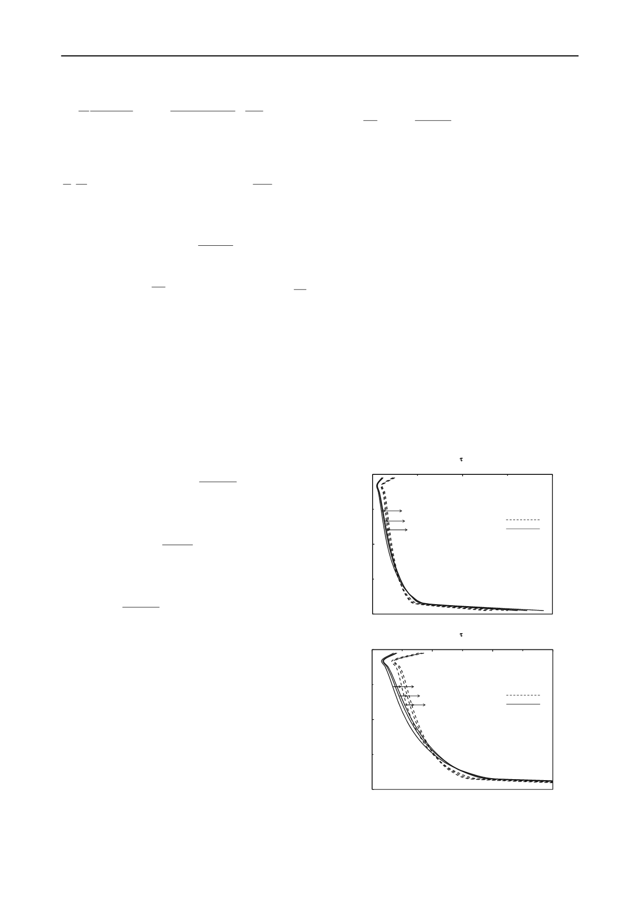
The influence of
s
on the variation of the shear stresses
with depth is presented in Figure 6 for L/d=10, K=50, ν
s
=0.5
and
gp
=0, 0.5 and 1. The variations of the shear stresses with
depth are magnified at top as shown in Figure 6(b). The
variations of shear stresses with depth are very similar for both
values of
s
= 0 and 0.5 and decrease with increasing values of
gp
. The shear stresses at the tip decrease from 6.65 to 5.63 and
from 5.25 to 4.39 for
s
= 0 & 0.5 with
gp
increasing from 0 to
1 respectively. On the contrary, the shear stresses at the top
increase from 0.35 to 0.41 and 0.77 to 0.86 for
s
= 0 & 0.5
with
gp
increasing from 0 to 1 respectively.
The variations of shear stresses with depth as a function of
gp
are presented in Figure 7 for L/d=10, K=50, ν
s
=0.5 and for
s
= 0, 0.5 and 1.0. The plots are magnified for the stresses at
the top in Figure 7(b). The variation of shear stresses with depth
for
gp
=0 & 0.5 are very similar for all
s
.
0.5
1
gp
=0
0
0.5
1
0
3.5
z/L
*
7
s
=0
s
=0.5
(a)
0.5
1
gp
=0
0
0.5
1
0
1
2
3
z/L
*
s
=0
s
=0.5
(b)
Fig. 6 Normalized shear stress,
*
vs. Depth, z/L for L/d = 10,
K=50 & ν
s
=0.5 – (a) Effect of
s
&
gp
.(b) Enlarged at top.


