2361
Technical Committee 209 /
Comité technique 209
0
1
2
3
4
5
6
7
0
1
2
3
4
5
6
7
8
Principal Stress ratio
=
1
/
3
Axial strain
1
(%)
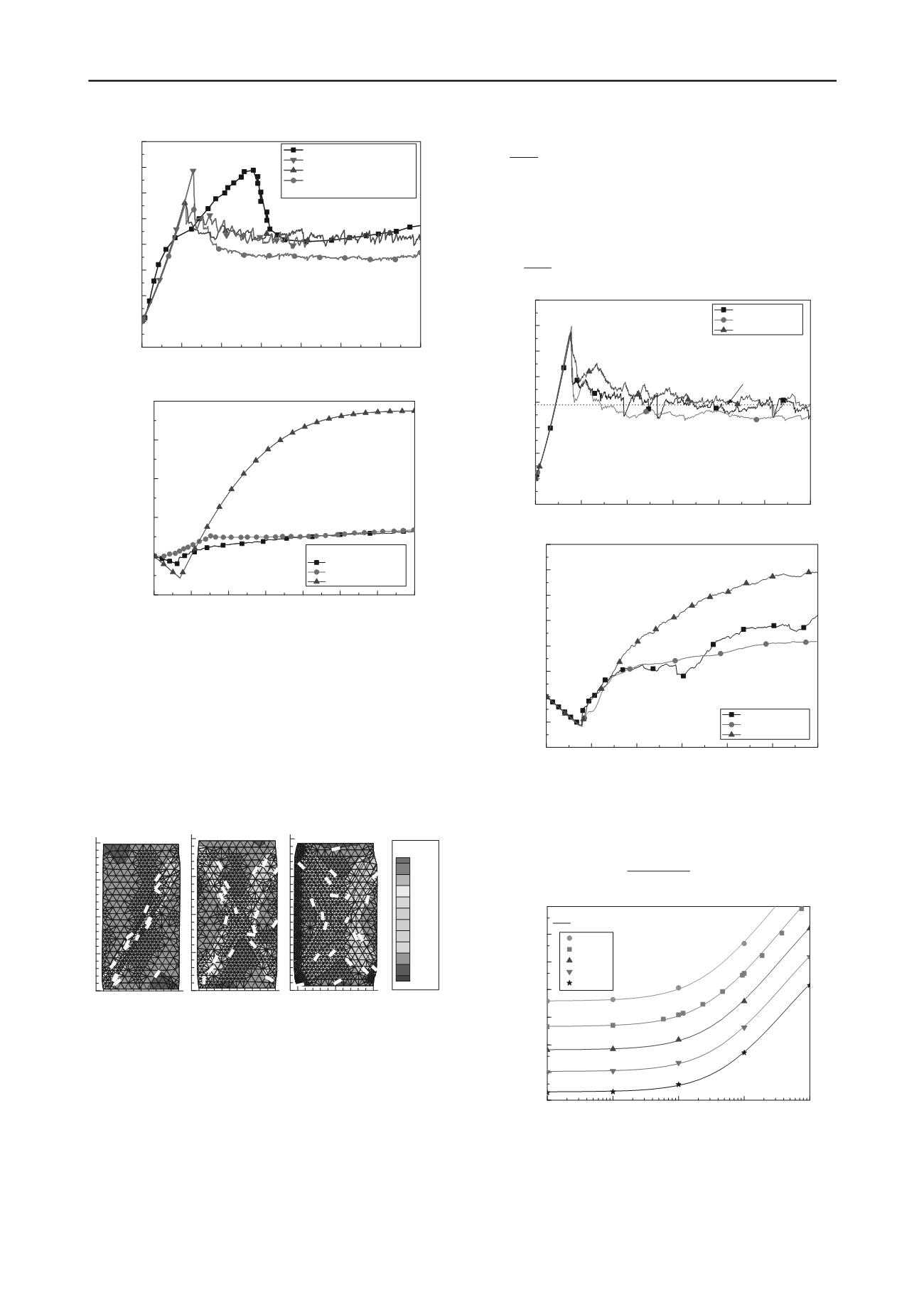
Laboratory drained biaxial test
Simulation A=0.60 (rough)
Simulation A=0.36 (rough)
Simulation A=0.36 (smooth)
Ottawa sand,
3
=69.4 kPa
Soil properties:
C
u
=1.4, D
50
=0.22mm, e
ini
=0.54, I
d
=0.87
Model parameters:
CSL: e
c
=0.64-0.014(p/101)
0.75
,
c
=36
o
Dilation: tan
=A(1-exp
sign(
)8|
|
0.75
)
Fig. 3 Biaxial test result of Ottawa sand simulated by FEM
0.00
0.02
0.04
0.06
0.08
0.10
0.12
0.14
0.04
0.00
-0.04
-0.08
-0.12
-0.16
Volumetric strain
v
Axial strain
1
Ottawa sand,
3
=69.4 kPa
Numerical bi-axial test
Laboratory bi-axial test
Single element test
Fig. 4
v
-
1
relation in biaxial test
Strain localization is critical in explaining some laboratory test
results where after the peak, the deviatoric stress,
q
, often decreases
to a stable value much earlier for axial strain than volume strain
(Samieh and Wong 1997; Salgado et al. 2000; Alshibli et al. 2003).
In Alshibli et al. (2003), the stress starts to oscillate around a stable
value after 10% axial strain, whilst the volume strain continuously
increases even over 25% axial strain. Once a “central” shear band
of soil at the critical state is formed, the apparent shear strength of
whole sample reaches the critical value. However the volume of
whole sample still increases with yielding of soil at the margins of
the shear band (Fig. 5).
0.52
0.54
0.54
0.54
0.54
0.56
0.56
0.56
0.56
0.58
0.58
0.58
0.58
0.6
0.6
0.6
0
50
100
0.52
0.54
0.54
0.54
0.54
0.54
0.54
0.56
0.56
0.56
0.56
0.56
0.56
0.56
0.56
0.58
0.58
0.58
0.6
0
50
100
0.52
0.52
0.54
0.54
0.54
0.54
0.56
0.56
0.56
0.56
0.56
0.58
0.58
0.58
0.58
0.58
0.58
0.58
0.6
0.6
0.6
0
50
100
e
0.7
0.68
0.66
0.64
0.62
0.6
0.58
0.56
0.54
0.52
0.5
Fig. 5 Void ratio field: (a)
1
=2%; (b)
1
=3%; (c)
1
=9%
The geometry of the specimen affects the shearing behavior.
Biaxial simulation results with different sample aspect ratios are
shown in Fig. 6. The
1
-
1
relation is nearly identical in all three
cases. However, the
v
-
1
relation is dependent on the aspect ratio of
the soil specimen and the shape of shear band formed.
5 BEARING CAPACITY OF A FOUNDATION ON SAND
The bearing capacity of circular plate on sand is analyzed by both
limit analysis (using the ABC program, Martin 2004) and LDFE. In
soil with self-weight the bearing capacity factor N
is often coupled
with N
q
although the two parts are not simply superposable. An N
q
-
N
bounding index
is defined as:
surf
D
q
(8)
where
D is a representative self-weight stress beneath the footing
and q
surf
is the surface surcharge. The coupled N
q
and N
bearing
capacity can be characterized by an integrated bearing capacity N
q
that varies with
and is defined as:
u
q
surf
q
N
q
(9)
0.00
0.01
0.02
0.03
0.04
0.05
0.06
0
1
2
3
4
5
6
7
8
Principal Stress ratio
=
1
/
3
Axial strain
1
100 X 300 Sample
100 X 200 Sample
100 X 100 Sample
Bi-axial test with fully rough boundary
e
ini
=0.54, I
d
=0.87,
c
=36
o
tan
=0.75(1-exp
sign(
)3.5|
|
0.75
)
c
= 3.85
(a)
1
-
1
relation
0.00
0.01
0.02
0.03
0.04
0.05
0.06
0.008
0.004
0.000
-0.004
-0.008
-0.012
-0.016
-0.020
-0.024
Volumetric strain
v
Axial strain
1
100 X 300 Sample
100 X 200 Sample
100 X 100 Sample
(b)
v
-
1
relation
Fig. 6 Effect of sample geometry on biaxial shearing behaviour
Limit analysis using ABC shows that the integrated N
q
factor for a
rough circular foundation can be approximated as (Fig. 7):
2 tan
(1 0.48 tan
)
1 0.0025
q
N e
(10)
0.01
0.1
1
10
100
8
16
32
64
128
256
512
1024
Integrated bearing capacity factor N
q
=q
u
/q
surf
Boundary condition
=
D/q
surf
=
=36
o
=
=32
o
=
=28
o
=
=24
o
=
=20
o
Limit analysis of circular plate penetration into sand
Best fit lines: N
q
=(1+0.48
tan
/(1+0.0025
))e
2
tan
Fig. 7 Coupled bearing capacity factor N
q
for a circular foundation
Referring to Fig. 7, the integrated N
q
factor approaches a constant
value with the decrease of the N
q
-N
bounding index
. That
ultimate value, e
2
tan
, can be regarded as N
q
. Similarly, the
integrated N
q
of rough strip foundation can be calculated as,


