2283
Technical Committee 208 /
Comité technique 208
(1)
where
p
= weighted mean probability of a particular damage
state being exceeded;
p
i
= the individual responses of the
probability of a particular damage state being exceeded;
E
i
= the
individual responses in terms of self-assessed experience; and
n
= the number of responses.
However, there does remain a question as to what a weighted
average means and statistical advice (Sexton, pers. comm.)
indicates that the results should be treated with a degree of
caution.
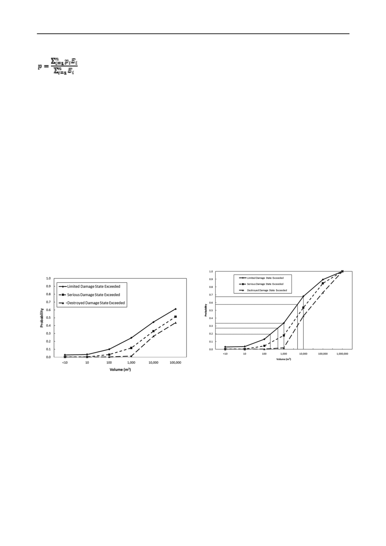
This yields fragility curves with lower probabilities of given
damage states being exceeded by a given event volume than
those derived from the full data set (Figure 2). This may
indicate that either those with less experience overestimate, or
those with greater expertise underestimate, potential damages.
The second approach involves rejecting the data from those
respondents reporting less experience, leaving only that from
those who assessed themselves as more experienced in this area.
Statistical advice (Sexton, Pers. Comm.) indicates that
approximately only scores from the upper 25% of the available
range should be examined. This implies that the analysis should
be undertaken for those judging their experience level as eight
or above (33% of respondents). However, plotting the data led
to a rather confused picture and to the conclusion that the 16
responses corresponding to the 33% of respondents reporting
their experience level to be eight or above were insufficient to
present a coherent picture. As for the weighting approach the
resulting fragility curves yield lower probabilities of given
damage states being exceeded by a given volume of event than
those derived from the full data set.
Figure 2. Weighted fragility curves: top, local roads; bottom, high
speed roads.
5 INTERPRETATION
The curves illustrated in Figure 1 do not stretch between zero
and unity. Even when manually extrapolated to a landslide
volume of 1,000,000m
3
the curves do not reach unity as would
be expected if they had been derived from by modelling in
which such an outcome would have been constrained.
Using the current approach it is inevitable that the mean
probability of each damage state being reached or exceeded is
less than unity unless all of the respondents return such a value.
This then begs the question of how to account for such an
inevitable, and seemingly contradictory, facet of the results. It is
straightforward to ‘force’ the curves to reach to unity by a ratio
approach (the forced probability at any value of landslide
volume,
p
if
=
p
i
.[1/
p
n
] where
p
i
is the mean probability and
p
n
is
the mean probability at the maximum landslide volume).
In order to determine whether such an approach can be
justified one must examine the more detailed responses of the
respondents to the questionnaire and in particular the responses
of those where a probability of unity was assigned to the
combinations of landslide volume and damage state. These data
illustrate, as might be anticipated, that the number of responses
assigning a probability of unity increases markedly with
landslide volume while decreasing with increased damage state
severity. Most importantly, for high landslide volumes, the
majority of respondents give unity for the likelihood of a given
damage state being reached or exceeded, lending justification to
‘forcing’ the curves to reach unity.
As discussed, the preliminary fragility curves of Figure 1 can
be forced to unity, and manually extrapolated to the next order
of magnitude in terms of landslide volume (i.e. 1,000,000m
3
).
The next logical step is to combine these two actions as
illustrated in Figure 3. The curves illustrated therein conform to
the ‘s’-shape generally perceived as being the correct form for
fragility curves. Notwithstanding this, one would normally
expect that the curves for different damage states would reach
unity at different landslide volumes; that they do not is a
function of the type of analysis undertaken and it seems
reasonable, as none of the curves reach unity, to force them all
to such a level at the highest volume considered.
Geographical variations and variations potentially caused by
respondents’ backgrounds (Academic, the Commercial Sector,
and Governments) were investigated. It was concluded that the
datasets were generally too small to draw definitive conclusions
albeit that the data appeared to suggest that:
Responses for the UK exhibited slightly higher probabilities
for larger landslide volumes compared to those for the ‘Rest
of the World’.
The responses for Academia exhibited slightly higher
probabilities for larger landslide volumes compared to those
for the Commercial Sector.
Figure 3. Fragility curves for high speed roads ‘forced’ to unity and
manually extrapolated to the next order of magnitude of debris flow
volume. Lines for Limited Damage at 200, 500, 1,000, 5,000 and
10,000m
3
are also shown.
6 VALIDATION
The comments received from respondents generally supported
the use of curves of the form illustrated in Figure 3 and events
from Scotland in the UK and the Republic of Korea are
considered here. Figure 4 illustrates hypothetically-shaped
curves in which the numbers given relate to a 5,000m
3
event on
a high speed road (Figure 3). The probabilities (
p
) of the
damage being equal to or greater than a given level are:
• Damage greater than or equal to ‘Limited’,
p
= 0.6.
• Damage greater than or equal to ‘Serious’,
p
= 0.4.
• Damage greater than or equal to ‘Destroyed’,
p
= 0.3.
The discrete, or conditional, damage state probabilities (i.e.
the probabilities of the occurrence of a given damage state) are
estimated from the probabilities given above:
• Probability of no damage = 1.0 - 0.6 = 0.4.
• Probability of ‘Limited’ damage = 0.6 – 0.4 = 0.2.
• Probability of ‘Serious’ damage = 0.4 – 0.3 = 0.1.
• Probability of ‘Destroyed’ damage state = 0.3.


